
Click on the top “Visual Learning for Beginners“, select “Star” or “Pin“
Essential content delivered to you first
 All algorithms in machine learning rely on minimizing or maximizing a certain function, which we call the objective function. The set of functions to be minimized is referred to as the loss function. The loss function measures the performance of the predictive model against the expected result. The most common method for finding the minimum of a function is gradient descent. Imagine the loss function as a hilly terrain; gradient descent is like sliding down from the top of the hill, aiming to reach the lowest point.No single loss function is suitable for all types of data. The choice of loss function depends on many factors, including the presence of outliers, the choice of machine learning algorithm, the time efficiency of running gradient descent, the ease of finding the derivative of the function, and the confidence in the predicted results. The purpose of this blog is to help you understand different loss functions.Loss functions can be broadly categorized into two types: classification loss and regression loss. The following article will focus on five types of regression loss.
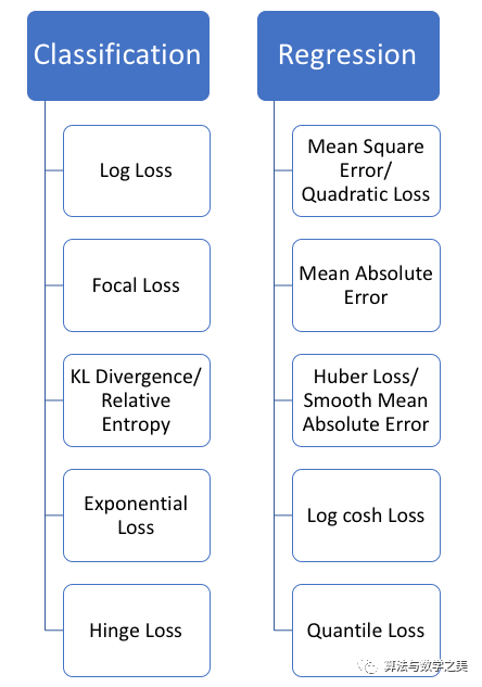 Regression functions predict real values, while classification functions predict labels
▌Regression Loss
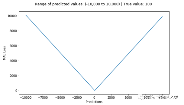
1. Mean Squared Error, Quadratic Loss, L2 Loss (Mean Square Error, Quadratic Loss, L2 Loss)Mean Squared Error (MSE) is the most commonly used regression loss function. MSE is the sum of the squared distances between the target variable and the predicted values.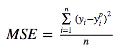 Here is a graph of the MSE function, where the true target value is 100, and the predicted values range from -10,000 to 10,000. When the predicted value (X-axis) equals 100, the MSE loss (Y-axis) reaches its minimum. The loss range is from 0 to ∞.
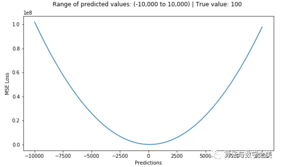 MSE Loss (Y-axis) vs Predicted Value (X-axis) Relationship Graph2. Mean Absolute Error, L1 Loss (Mean Absolute Error, L1 Loss)Mean Absolute Error (MAE) is another loss function used for regression models. MAE is the sum of the absolute differences between the target variable and the predicted variable. Therefore, it measures the average magnitude of errors in a set of predictions without considering the direction of the errors. (If we also consider direction, it would be called Mean Bias Error (MBE), which is the sum of the residuals or errors). The loss range is also from 0 to ∞.
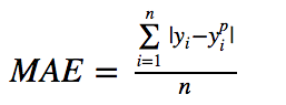
 MAE Loss (Y-axis) vs Predicted Value (X-axis) Relationship Graph3. MSE vs MAE (L2 Loss vs L1 Loss)In short, using squared error is easier to solve, but using absolute error is more robust to outliers. However, knowing the reason behind it is just as important!Whenever we train a machine learning model, our goal is to find the point that minimizes the loss function. Of course, both loss functions reach their minimum when the predicted value exactly equals the true value.Now, let’s quickly go through the Python code for both loss functions. We can either write our own functions or use the built-in metric functions from sklearn:
# true: array of true target variable
# pred: predicted array

def mse(true, pred):
   return np.sum(((true - pred)**2))

def mae(true, pred):
   return np.sum(np.abs(true - pred))

# Also can be used in sklearn
from sklearn.metrics import mean_squared_error
from sklearn.metrics import mean_absolute_error
Let’s take a look at the MAE and RMSE values (RMSE, Root Mean Square Error, which is just the square root of MSE to make it comparable to the range of MAE) for two examples. In the first example, the predicted values are close to the true values, and the variance of the errors between observations is small. In the second example, there is an outlier observation, resulting in a high error.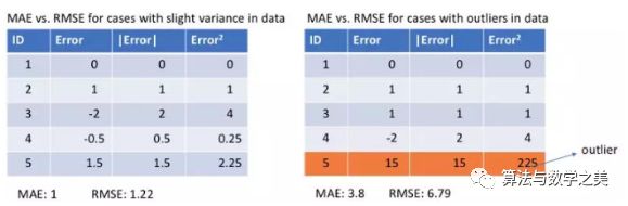 Left: Errors are close to each other Right: An error is far from the othersWhat do we observe from this? How should we choose which loss function to use?Since MSE squares the errors (e) (y – y_predicted = e), if e > 1, the value of the error increases significantly. If we have an outlier in our data, the value of e will be very high and will far exceed |e|. This means that a model using MSE as a loss will give much higher weight to outliers compared to a model using MAE. In the second example above, a model using RMSE as a loss will adjust to minimize this outlier, but at the cost of sacrificing the predictive performance of other normal data points, ultimately reducing the overall performance of the model.MAE loss is suitable when the training data is corrupted by outliers (i.e., when we erroneously obtain unrealistic large positive or negative values in the training data rather than the test data).Intuitively, we can think of it this way: for all observed data, if we only give one predicted result to minimize MSE, then that prediction should be the mean of all target values. However, if we try to minimize MAE, then this prediction is the median of all target values. We know that the median is more robust to outliers than the mean, which makes MAE more robust than MSE.A significant issue with using MAE loss (especially for neural networks) is that its gradient is always the same, meaning that even for small loss values, its gradient is large. This is not good for the model’s learning. To address this issue, we can use a dynamic learning rate that decreases as we approach the minimum. MSE performs well in this case, even with a fixed learning rate it will converge. The gradient of the MSE loss is larger when the loss value is high and decreases as the loss approaches 0, making it more precise at the end of training (see the graph below).
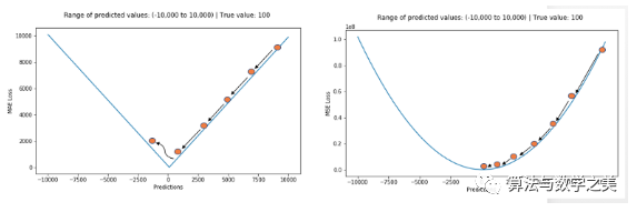 Deciding Which Loss Function to Use?If outliers affect the business and should be detected as anomalies, then we should use MSE. On the other hand, if we believe that outliers merely represent corrupted data, then we should choose MAE as the loss.I recommend reading the article below, which has a great study comparing the performance of regression models using L1 loss and L2 loss in the presence and absence of outliers. Remember, L1 and L2 losses are just another name for MAE and MSE respectively.
Address:http://rishy.github.io/ml/2015/07/28/l1-vs-l2-loss/
L1 loss is more robust to outliers, but its derivative is not continuous, making it less efficient to solve. L2 loss is sensitive to outliers but provides a more stable closed-form solution (by setting its derivative to 0).Both loss functions have their issues: it may happen that neither loss function can provide ideal predictions. For example, if 90% of the true target values in our data are 150, while the remaining 10% have true target values between 0-30, then a model using MAE as a loss might predict all observations as 150, ignoring the 10% outlier cases because it will try to approach the median. Similarly, a model using MSE as a loss will give many predictions ranging from 0 to 30 because it gets confused by the outliers. Both outcomes are undesirable in many businesses.What to do in such cases? A simple solution is to transform the target variable. Another approach is to try different loss functions. This is the motivation behind our third loss function—Huber Loss.3. Huber Loss, Smooth Mean Absolute ErrorHuber Loss is less sensitive to outliers than squared error loss. It is also differentiable at 0. Essentially, it is the absolute error, which is quadratic when the error is small. When the error needs to become quadratic depends on a hyperparameter, (delta), which can be fine-tuned. When 𝛿 ~ 0, Huber Loss approaches MAE, and when 𝛿 ~ ∞ (a large number), Huber Loss approaches MSE.
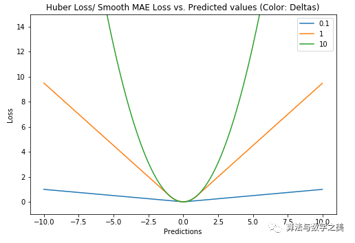 Huber Loss (Y-axis) vs Predicted Value (X-axis) Relationship Graph. True Value = 0The choice of delta is very important, as it determines what data you consider as outliers. Residuals greater than delta are minimized with L1 (less sensitive to larger outliers), while residuals less than delta can be “suitably” minimized with L2.Why Use Huber Loss?A significant issue with using MAE to train neural networks is that we often encounter large gradients, which can cause the training to miss the minimum when using gradient descent. For MSE, the gradient decreases as the loss approaches the minimum, making it more precise.In this case, Huber Loss can be very useful as it curves near the minimum, thus reducing the gradient. Additionally, it is more robust to outliers than MSE. Therefore, it combines the best features of MSE and MAE. However, the issue with Huber Loss is that we may need to iteratively train the hyperparameter delta.4. Log-Cosh LossLog-Cosh is another loss function for regression tasks that is smoother than L2. Log-Cosh is the logarithm of the hyperbolic cosine of the prediction error.
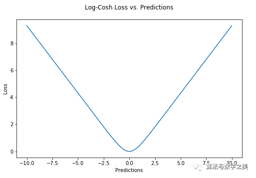
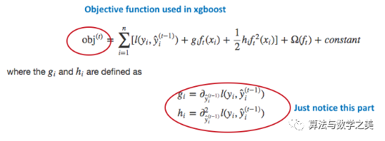 XGBoost Target Function Used. Note Its Dependence on First and Second Derivatives.However, Log-Cosh Loss is not perfect. It still has gradient and Hessian issues; for predictions with large errors, its gradient and Hessian are constant. This can lead to no splits in XGBoost.Python code for Huber and Log-Cosh loss functions:
def sm_mae(true, pred, delta):
   """
   true: array of true values
   pred: array of predicted values

   returns: smoothed mean absolute error loss
   """
   loss = np.where(np.abs(true-pred) < delta , 0.5*((true-pred)**2), delta*np.abs(true - pred) - 0.5*(delta**2))
   return np.sum(loss)

def logcosh(true, pred):
   loss = np.log(np.cosh(pred - true))
   return np.sum(loss)
5. Quantile LossIn most real prediction problems, we usually want to understand the uncertainty of our predictions. Understanding the range of predicted values rather than just a single prediction point can significantly improve decision-making processes for many business issues.When we are interested in predicting an interval rather than just a point prediction, the Quantile Loss function becomes useful. The prediction intervals of least squares regression are based on the assumption that the residuals (y – y_hat) have constant variance across the values of the independent variables. We cannot trust linear regression models because they violate this assumption. Of course, we cannot simply assume that using nonlinear functions or tree-based models will better model this situation; we must still consider fitting a linear regression model as a baseline. This is where Quantile Loss comes into play, as regression models based on Quantile Loss can provide reasonable prediction intervals, even for residuals with non-constant variance or non-normal distribution.Let’s look at an effective example to better understand why regression models based on Quantile Loss perform well on heteroscedastic data.Quantile Regression vs Ordinary Least Squares (OLS) Regression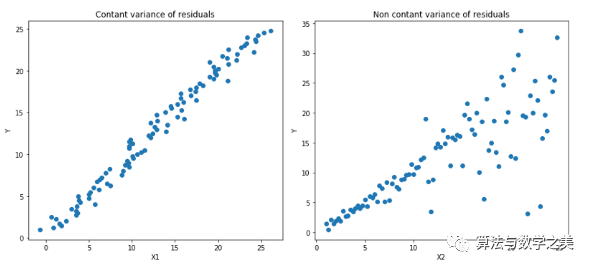 Left: Linear relationship between X1 and Y, with constant variance of residuals. Right: Linear relationship between X2 and Y, but the variance of Y increases as X2 increases (heteroscedastic).
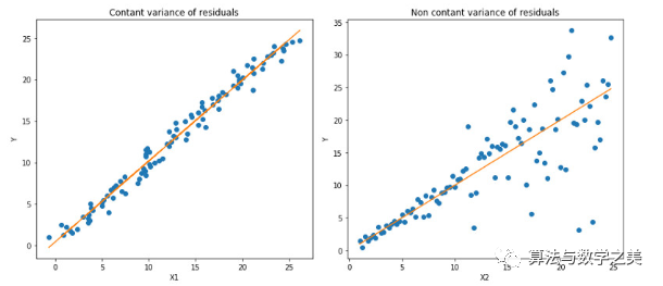 The orange line indicates the OLS estimates in both cases.
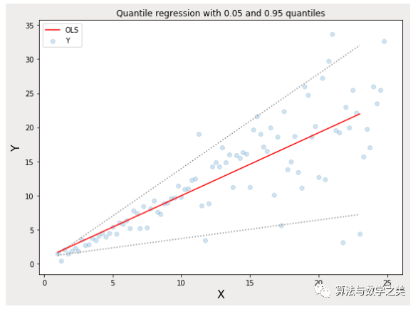 Quantile Regression: The dashed lines indicate regression estimates based on the 0.05 and 0.95 quantile loss functions.The Quantile regression code shown above is available in the notebook below.
Address:https://github.com/groverpr/Machine-Learning/blob/master/notebooks/09_Quantile_Regression.ipynb
Understanding the Quantile Loss FunctionThe purpose of Quantile regression is to estimate the conditional “quantiles” of the dependent variable given certain values of the predictor variables. Quantile Loss is essentially an extension of MAE (when the quantile is the 50th percentile, Quantile Loss degenerates to MAE).The idea behind Quantile Loss is to choose the quantile value based on whether we want to give more weight to overestimation or underestimation. The loss function penalizes overestimated and underestimated predicted values differently based on the chosen quantile (γ) value. For example, a Quantile Loss function with γ = 0.25 gives more penalty to overestimated predicted values and tries to make the predicted values slightly lower than the median.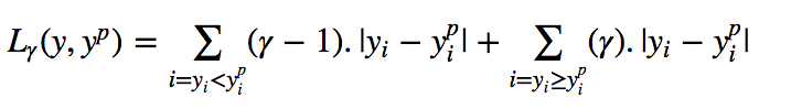 γ is the given quantile, which ranges between 0 and 1.
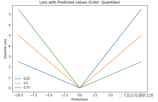 Quantile Loss (Y-axis) vs Predicted Value (X-axis) Relationship Graph. True Value is Y= 0We can also use this loss function to calculate the prediction intervals for neural networks or tree-based models. The following figure shows the prediction intervals calculated using the quantile loss function in the gradient boosting tree.
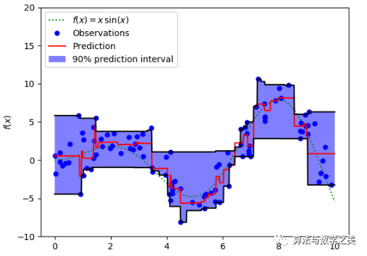 Prediction Intervals Using Quantile Loss (Gradient Boosting Regression)The above figure shows the 90% prediction intervals calculated using the quantile loss function in the GradientBoostingRegression of the sklearn library. The upper limit is calculated using γ = 0.95, while the lower limit uses γ = 0.05.
▌Comparative Study
“Gradient boosting machines, a tutorial” provides a great comparative study. To demonstrate the properties of all the above loss functions, researchers created an artificial dataset sampled from the sinc(x) function, which included two types of artificial noise: Gaussian noise component and impulse noise component. The impulse noise term is used to demonstrate the robustness of the results. Below are the results of fitting GBM (Gradient Boosting Machine) using different loss functions.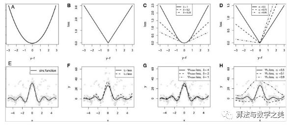 Continuous loss functions: (A) MSE loss function; (B) MAE loss function; (C) Huber loss function; (D) Quantile loss function. Example of fitting a smooth GBM with noisy sinc(x) data: (E) Original sinc(x) function; (F) Smooth GBM fitted with MSE and MAE as losses; (G) Smooth GBM fitted with Huber Loss, = {4,2,1}; (H) Smooth GBM fitted with Quantile Loss.Some observations from the simulated experiment:
-
The model using MAE as a loss is less affected by impulse noise, while the model using MSE as a loss is slightly biased due to data deviations caused by impulse noise.
-
The model using Huber Loss as a loss function is less sensitive to the chosen hyperparameters.
-
Quantile Loss provides good estimates for the corresponding confidence levels.
A graph illustrating all loss functions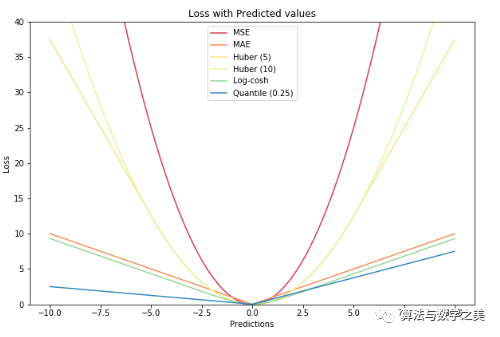
Good news!
Visual Learning for Beginners Knowledge Circle
Is now open to the public👇👇👇


Download 1: OpenCV-Contrib Extension Module Chinese Tutorial
Reply "Chinese Tutorial for Extension Modules" in the "Visual Learning for Beginners" public account background to download the first Chinese version of the OpenCV extension module tutorial on the internet, covering installation of extension modules, SFM algorithms, stereo vision, target tracking, biological vision, super-resolution processing, etc. over twenty chapters of content.

Download 2: Python Vision Practical Project 52 Lectures
Reply "Python Vision Practical Project" in the "Visual Learning for Beginners" public account background to download 31 visual practical projects including image segmentation, mask detection, lane line detection, vehicle counting, adding eyeliner, license plate recognition, character recognition, emotion detection, text content extraction, facial recognition, etc., to help quickly learn computer vision.

Download 3: OpenCV Practical Project 20 Lectures
Reply "OpenCV Practical Project 20 Lectures" in the "Visual Learning for Beginners" public account background to download 20 practical projects based on OpenCV, achieving advanced learning of OpenCV.

Discussion Group

Welcome to join the reader group of the public account to communicate with peers. Currently, there are WeChat groups on SLAM, 3D vision, sensors, autonomous driving, computational photography, detection, segmentation, recognition, medical imaging, GAN, algorithm competitions, etc. (will be gradually subdivided in the future). Please scan the WeChat number below to join the group, with the note: "Nickname + School/Company + Research Direction", for example: "Zhang San + Shanghai Jiao Tong University + Visual SLAM". Please follow the format for notes, otherwise, you will not be approved. After successfully added, you will be invited to the relevant WeChat group based on your research direction. Please do not send advertisements in the group, otherwise you will be removed from the group, thank you for your understanding~