
Source: DeepHub IMBA


This article is about 6000 words long and is recommended to be read in 10+ minutes.
This article will first explore mixture models, focusing on Gaussian mixture models and their fundamental principles.
Gaussian Mixture Model (GMM) is a statistical model that represents data as a mixture of Gaussian (normal) distributions. These models can be used to identify groups within a dataset and capture the complex, multimodal structure of data distributions.
GMM can be applied in various machine learning tasks, including clustering, density estimation, and pattern recognition.
In this article, we will first discuss mixture models, with a focus on Gaussian mixture models and their fundamental principles. We will then explore how to estimate the parameters of these models using a powerful technique called Expectation-Maximization (EM) and provide an implementation from scratch in Python. Finally, we will demonstrate how to perform clustering using GMM with the Scikit-Learn library.
Mixture Models
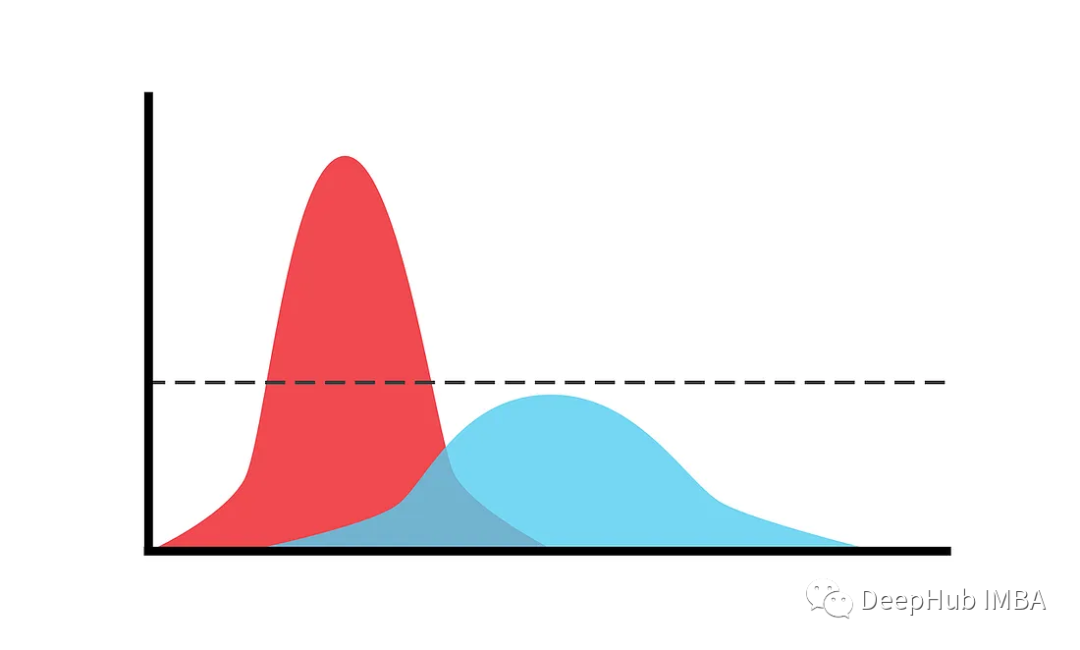
Mixture models are probabilistic models used to represent data that may come from multiple different sources or categories, each modeled by a separate probability distribution. For example, financial returns often exhibit different behaviors under normal market conditions and during crises, and can thus be modeled as a mixture of two different distributions.
Formally, if X is a random variable whose distribution is a mixture of K component distributions, then the probability density function (PDF) or probability mass function (PMF) of X can be expressed as:

P (x) is the total density or mass function of the mixture model. K is the number of component distributions in the mixture model.
fₖ(x;θₖ) is the density or mass function of the k-th component distribution, parameterized by θₖ.
Wₖ is the mixing weight of the k-th component, where 0≤Wₖ≤1 and the sum of weights equals 1. Wₖ is also known as the prior probability of component k.
θₖ represents the parameters of the k-th component, such as the mean and standard deviation in a Gaussian distribution.
The mixture model assumes that each data point comes from one of the K component distributions, selected according to the mixing weights wₖ. The model does not require knowledge of which distribution each data point belongs to.
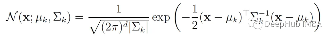
Gaussian Mixture Model (GMM) is a common mixture model whose probability density is given by a mixture of Gaussian distributions:

X is a d-dimensional vector.
μₖ is the mean vector of the k-th Gaussian component.
Σₖ is the covariance matrix of the k-th Gaussian component.
N (x;μₖ,Σₖ) is the multivariate normal density function of the k-th component:
For univariate Gaussian distribution, the probability density can be simplified to:

μₖ is the mean of the k-th Gaussian component.
σₖ is the covariance matrix of the k-th Gaussian component.
N (x;μₖ,σₖ) is the univariate normal density function of the k-th component:

The following Python function plots the mixture distribution of two univariate Gaussian distributions:
from scipy.stats import norm def plot_mixture(mean1, std1, mean2, std2, w1, w2): # Generate points for the x-axis x = np.linspace(-5, 10, 1000) # Calculate the individual normal distributions normal1 = norm.pdf(x, mean1, std1) normal2 = norm.pdf(x, mean2, std2) # Calculate the mixture mixture = w1 * normal1 + w2 * normal2 # Plot the results plt.plot(x, normal1, label='Normal distribution 1', linestyle='--') plt.plot(x, normal2, label='Normal distribution 2', linestyle='--') plt.plot(x, mixture, label='Mixture model', color='black') plt.xlabel('$x$') plt.ylabel('$p(x)$') plt.legend()
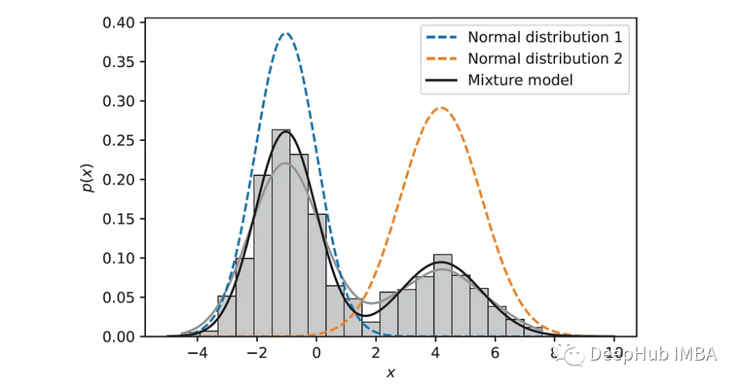
We use this function to plot the mixture of two Gaussian distributions with parameters μ₁= -1, σ₁= 1, μ₂= 4, σ₂= 1.5, and mixing weights w₁= 0.7 and w₂= 0.3:
# Parameters for the two univariate normal distributions mean1, std1 = -1, 1 mean2, std2 = 4, 1.5 w1, w2 = 0.7, 0.3 plot_mixture(mean1, std1, mean2, std2, w1, w2)
The dashed lines represent the individual normal distributions, and the black solid line represents the mixture result. This plot illustrates how the mixture model combines two distributions, each with its own mean, standard deviation, and weight in the overall mixture result.
Learning GMM Parameters
The goal of our learning is to find the GMM parameters (means, covariances, and mixing coefficients) that best explain the observed data. To do this, we first need to define the likelihood of the model given the input data.
For a GMM with K components, the dataset X = {X 1, …, X n} (n data points), the likelihood function L is given by the product of the probability densities of each data point, defined by the GMM:

Where θ represents all the parameters of the model (means, variances, and mixing weights).
In practice, it is easier to work with log-likelihood because the product of probabilities can lead to numerical underflow for large datasets. The log-likelihood is given by:
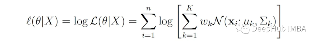
The parameters of the GMM can be estimated by maximizing the log-likelihood function with respect to θ. However, we cannot directly apply Maximum Likelihood Estimation (MLE) to estimate the parameters of the GMM:
The log-likelihood function is highly nonlinear and difficult to maximize analytically.
The model has latent variables (mixing weights) that cannot be directly observed in the data.
To overcome these issues, the Expectation-Maximization (EM) algorithm is typically used to solve the problem.
Expectation-Maximization (EM)
The EM algorithm is a powerful method for finding maximum likelihood estimates of parameters in statistical models that depend on unobserved latent variables.
The algorithm first randomly initializes the model parameters. It then iterates between two steps:
1. Expectation Step (E-step): Calculate the expected log-likelihood of the model with respect to the distribution of the latent variables based on the observed data and the current estimates of the model parameters. This step involves estimating the probabilities of the latent variables.
2. Maximization Step (M-step): Update the model parameters to maximize the log-likelihood of the observed data, given the estimates of the latent variables from the E-step.
These two steps are repeated until convergence, typically determined by a threshold of change in log-likelihood or a maximum number of iterations.
In GMMs, the latent variables represent the unknown component membership of each data point. Let Z′ be a random variable representing the component that generated the data point x′. Z′ can take a value from {1, …, K}, corresponding to the K components.
E-Step
In the E-step, we calculate the probability distribution of the latent variable Z ^ based on the current estimates of the model parameters. In other words, we compute the membership probability of each data point in each Gaussian component.
The probability that Z′= k, meaning x′ belongs to the k-th component, can be computed using Bayes’ rule:
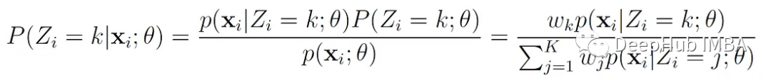
We denote this probability with the variable γ(z′ₖ), and it can be expressed as:

The variable γ(z′ₖ) is often referred to as responsibilities because it describes the responsibilities of each component for each observation. These parameters serve as proxies for the missing information about the latent variables.
The expected log-likelihood regarding the distribution of the latent variables can now be expressed as:

The function Q is the weighted sum of the log-likelihoods of all data points under each Gaussian component, where the weights are the responsibilities we mentioned above. Q differs from the previously shown log-likelihood function l(θ|X). The log-likelihood l(θ|X) represents the likelihood of the observed data under the entire mixture model without explicitly considering the latent variables, whereas Q represents the expected log-likelihood of the observed data and the estimated distribution of the latent variables.
M-Step
In the M-step, we update the parameters θ (means, covariances, and mixing weights) of the GMM to maximize the expected likelihood Q(θ) computed in the E-step.
The parameter updates are as follows:
1. Updating each component:

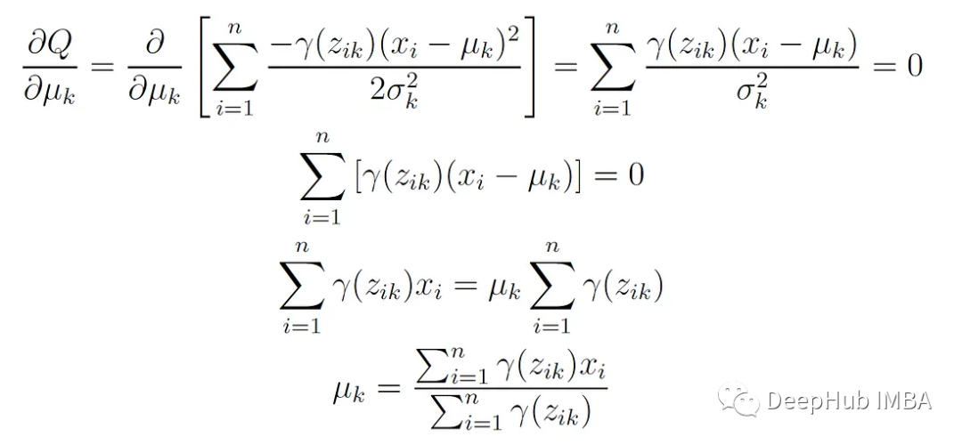
The new mean of the k-th component is the weighted average of all data points, where the weights are the probabilities of those points belonging to component k. This update formula can be obtained by maximizing the expected log-likelihood function Q with respect to the mean μₖ.
Here are the proof steps; the expected log-likelihood for univariate Gaussian distribution is:

This function is differentiated with respect to μₖ and set to 0, yielding:
2. Update the covariance of each component:

That is, the new covariance of the k-th component is the weighted average of the squared deviations of each data point from the mean of that component, where the weights are the probabilities assigned to that component.
In the case of univariate normal distribution, this update simplifies to:

3. Update the mixing weights:

That is, the new weight of the k-th component is the total probability of the points belonging to that component, normalized by the number of points n.
Repeating these two steps ensures convergence to a local maximum of the likelihood function. Since the final optimum depends on the initial random parameter values, a common practice is to run the EM algorithm multiple times with different random initializations and keep the model that achieves the highest likelihood.
Python Implementation
Next, we will implement the EM algorithm in Python to estimate the parameters of a GMM for two univariate Gaussian distributions from a given dataset.
First, we import the necessary libraries:
 import numpy as np import matplotlib.pyplot as plt import seaborn as sns  from scipy.stats import norm  np.random.seed(0) # for reproducibility

Next, let’s write a function to initialize the GMM parameters:
def init_params(x): """Initialize the parameters for the GMM """ # Randomly initialize the means to points from the dataset mean1, mean2 = np.random.choice(x, 2, replace=False) # Initialize the standard deviations to 1 std1, std2 = 1, 1 # Initialize the mixing weights uniformly w1, w2 = 0.5, 0.5 return mean1, mean2, std1, std2, w1, w2
The means are initialized from random data points in the dataset, the standard deviations are set to 1, and the mixing weights are set to 0.5.
In the E-step, we compute the probabilities of each data point belonging to each Gaussian component:
def e_step(x, mean1, std1, mean2, std2, w1, w2): """E-Step: Compute the responsibilities """ # Compute the densities of the points under the two normal distributions prob1 = norm(mean1, std1).pdf(x) * w1 prob2 = norm(mean2, std2).pdf(x) * w2 # Normalize the probabilities prob_sum = prob1 + prob2 prob1 /= prob_sum prob2 /= prob_sum return prob1, prob2
In the M-step, we update the model parameters based on the calculations from the E-step:
def m_step(x, prob1, prob2): """M-Step: Update the GMM parameters """ # Update means mean1 = np.dot(prob1, x) / np.sum(prob1) mean2 = np.dot(prob2, x) / np.sum(prob2) # Update standard deviations std1 = np.sqrt(np.dot(prob1, (x - mean1)**2) / np.sum(prob1)) std2 = np.sqrt(np.dot(prob2, (x - mean2)**2) / np.sum(prob2)) # Update mixing weights w1 = np.sum(prob1) / len(x) w2 = 1 - w1 return mean1, std1, mean2, std2, w1, w2
Finally, we write the main function to run the EM algorithm, iterating between the E-step and M-step for a specified number of iterations:
def gmm_em(x, max_iter=100): """Gaussian mixture model estimation using Expectation-Maximization """ mean1, mean2, std1, std2, w1, w2 = init_params(x) for i in range(max_iter): print(f'Iteration {i}: μ1 = {mean1:.3f}, σ1 = {std1:.3f}, μ2 = {mean2:.3f}, σ2 = {std2:.3f}, ' f'w1 = {w1:.3f}, w2 = {w2:.3f}') prob1, prob2 = e_step(x, mean1, std1, mean2, std2, w1, w2) mean1, std1, mean2, std2, w1, w2 = m_step(x, prob1, prob2) return mean1, std1, mean2, std2, w1, w2
To test our implementation, we need to create a synthetic dataset by sampling from a known mixture distribution with predefined parameters. We will then use the EM algorithm to estimate the parameters of the distribution and compare the estimated parameters with the original ones.
First, we sample data from a mixture of two univariate normal distributions:
def sample_data(mean1, std1, mean2, std2, w1, w2, n_samples): """Sample random data from a mixture of two Gaussian distribution. """ x = np.zeros(n_samples) for i in range(n_samples): # Choose distribution based on mixing weights if np.random.rand() < w1: # Sample from the first distribution x[i] = np.random.normal(mean1, std1) else: # Sample from the second distribution x[i] = np.random.normal(mean2, std2) return x
Then we use this function to sample 1000 data points from the previously defined mixture:
Now we can run the EM algorithm on this dataset:
final_dist_params = gmm_em(x, max_iter=30)We obtain the following output:
Iteration 0: μ1 = -1.311, σ1 = 1.000, μ2 = 0.239, σ2 = 1.000, w1 = 0.500, w2 = 0.500 Iteration 1: μ1 = -1.442, σ1 = 0.898, μ2 = 2.232, σ2 = 2.521, w1 = 0.427, w2 = 0.573 Iteration 2: μ1 = -1.306, σ1 = 0.837, μ2 = 2.410, σ2 = 2.577, w1 = 0.470, w2 = 0.530 Iteration 3: μ1 = -1.254, σ1 = 0.835, μ2 = 2.572, σ2 = 2.559, w1 = 0.499, w2 = 0.501 ... Iteration 27: μ1 = -1.031, σ1 = 1.033, μ2 = 4.180, σ2 = 1.371, w1 = 0.675, w2 = 0.325 Iteration 28: μ1 = -1.031, σ1 = 1.033, μ2 = 4.181, σ2 = 1.370, w1 = 0.675, w2 = 0.325 Iteration 29: μ1 = -1.031, σ1 = 1.033, μ2 = 4.181, σ2 = 1.370, w1 = 0.675, w2 = 0.325The algorithm converged to parameters close to the original ones: μ₁= -1.031, σ₁= 1.033, μ₂= 4.181, σ₂= 1.370, mixing weights w₁= 0.675, w₂= 0.325.
Let’s use the previously written plot_mixture() function to plot the final distribution and the histogram of the sampled data:
def plot_mixture(x, mean1, std1, mean2, std2, w1, w2): # Plot a histogram of the input data sns.histplot(x, bins=20, kde=True, stat='density', linewidth=0.5, color='gray') # Generate points for the x-axis x_ = np.linspace(-5, 10, 1000) # Calculate the individual normal distributions normal1 = norm.pdf(x_, mean1, std1) normal2 = norm.pdf(x_, mean2, std2) # Calculate the mixture mixture = w1 * normal1 + w2 * normal2 # Plot the results plt.plot(x_, normal1, label='Normal distribution 1', linestyle='--') plt.plot(x_, normal2, label='Normal distribution 2', linestyle='--') plt.plot(x_, mixture, label='Mixture model', color='black') plt.xlabel('$x$') plt.ylabel('$p(x)$') plt.legend() plot_mixture(x, *final_dist_params)The result is shown in the figure below:
It is evident that the estimated distribution closely matches the histogram of the data points. The above Python code is provided for our understanding of the algorithm, but in practical applications, many issues may arise. Therefore, for actual use, one can directly utilize the implementation in Scikit-Learn.
GMM in Scikit-Learn
Scikit-Learn provides an implementation of Gaussian Mixture Models in the class sklearn.mixture.GaussianMixture.
Unlike other clustering algorithms in Scikit-Learn, this algorithm does not provide the labels_ attribute. Therefore, to obtain the clustering assignments of data points, you need to call the predict() method on the fitted model (or call fit_predict()).
Below, we will use this class to perform clustering on a dataset consisting of two elliptical blobs and one spherical blob:
 from sklearn.datasets import make_blobs  X, y = make_blobs(n_samples=500, centers=[(0, 0), (4, 4)], random_state=0)  # Apply a linear transformation to make the blobs elliptical transformation = [[0.6, -0.6], [-0.2, 0.8]] X = np.dot(X, transformation)  # Add another spherical blob X2, y2 = make_blobs(n_samples=150, centers=[(-2, -2)], cluster_std=0.5, random_state=0) X = np.vstack((X, X2))

Let’s take a look at our data:
def plot_data(X): sns.scatterplot(x=X[:, 0], y=X[:, 1], edgecolor='k', legend=False) plt.xlabel('$x_1$') plt.ylabel('$x_2$') plot_data(X)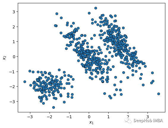
Next, we instantiate the GMM class with n_components=3 and call its fit_predict() method to obtain the cluster assignments:
 from sklearn.mixture import GaussianMixture  gmm = GaussianMixture(n_components=3) labels = gmm.fit_predict(X)

You can check how many iterations the EM algorithm needed to converge:
print(gmm.n_iter_) 2The EM algorithm converged in just two iterations. Let’s check the estimated GMM parameters:
 print('Weights:', gmm.weights_) print('Means:
', gmm.means_) print('Covariances:
', gmm.covariances_)
The results are as follows:
Weights: [0.23077331 0.38468283 0.38454386] Means: [[-2.01578902 -1.95662033] [-0.03230299 0.03527593] [ 1.56421574 0.80307925]] Covariances: [[[ 0.254315 -0.01588303] [-0.01588303 0.24474151]] [[ 0.41202765 -0.53078979] [-0.53078979 0.99966631]] [[ 0.35577946 -0.48222654] [-0.48222654 0.98318187]]]It can be seen that the estimated weights are very close to the original proportions of the three blobs, and the means and variances of the spherical blob are very close to its original parameters.
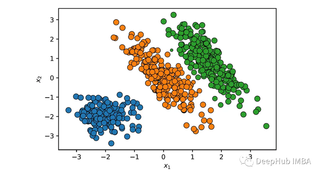
Let’s plot the results of the clustering:
def plot_clusters(X, labels): sns.scatterplot(x=X[:, 0], y=X[:, 1], hue=labels, palette='tab10', edgecolor='k', legend=False) plt.xlabel('$x_1$') plt.ylabel('$x_2$') plot_clusters(X, labels)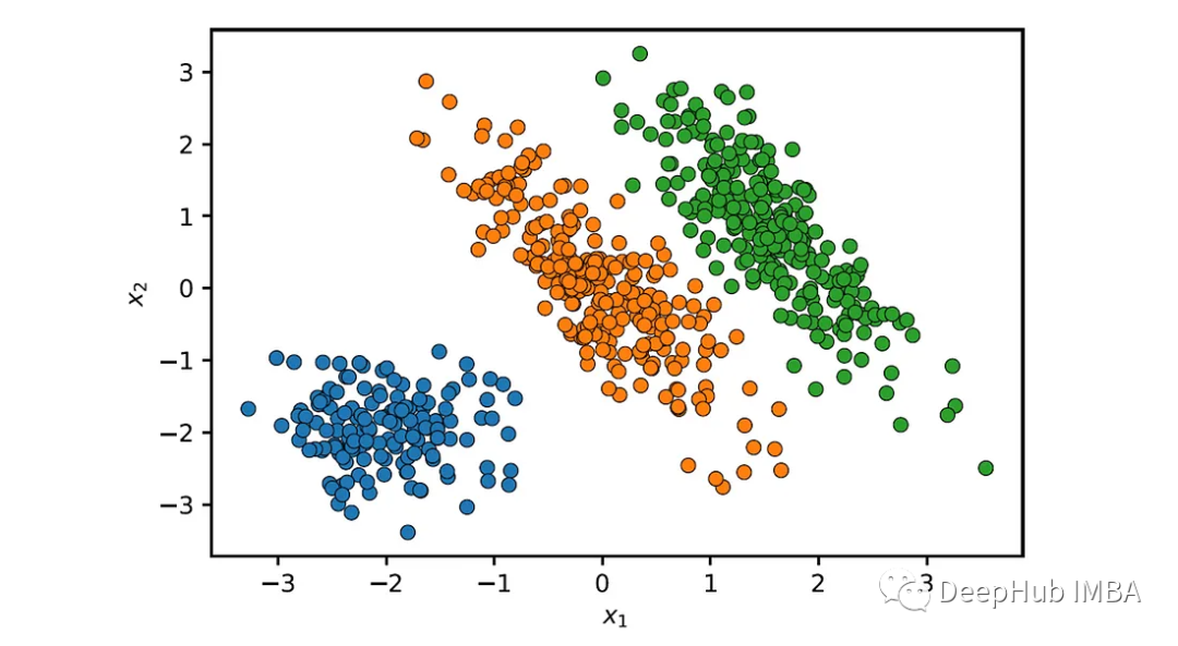
GMM correctly identified these three clusters.
We can also use the predict_proba() method to obtain the membership probabilities of each data point in each cluster.
prob = gmm.predict_proba(X)For example, the probability that the first point in the dataset belongs to the green cluster is very high:
print('x =', X[0]) print('prob =', prob[0]) #x = [ 2.41692591 -0.07769481] #prob = [3.11052582e-21 8.85973054e-10 9.99999999e-01]We can visualize these probabilities by making the size of each point proportional to the probability that it belongs to the cluster it was assigned to:
Points located on the boundary between the two elliptical clusters have lower probabilities. Data points with significantly low probability densities (e.g., below a predefined threshold) can be identified as anomalies or outliers.
We can also compare with other clustering methods:
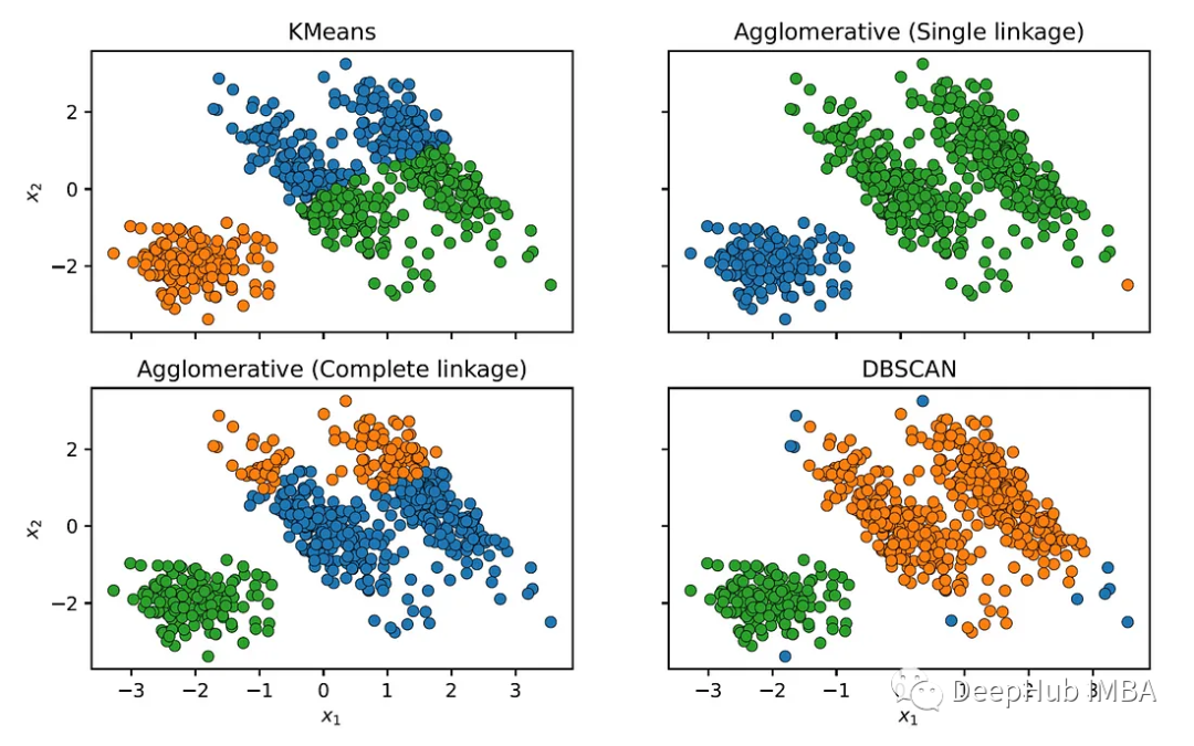
It can be seen that other clustering algorithms fail to correctly identify the elliptical clusters.
Model Evaluation
Log-likelihood is the primary method for evaluating GMMs. It can also be monitored during training to check the convergence of the EM algorithm. To compare models with different numbers of components or different covariance structures, two additional metrics are needed that balance model complexity (number of parameters) and goodness of fit (represented by log-likelihood):
1. Akaike Information Criterion (AIC):

P is the number of parameters in the model (including all means, covariances, and mixing weights). L is the likelihood of the model (likelihood of the model with optimal parameter values).
The lower the AIC value, the better the model. AIC rewards models that fit the data well but penalizes models with more parameters.
2. Bayesian Information Criterion (BIC):

In this case, the definitions of p and L are the same as before, and n is the number of data points.
Like AIC, BIC balances model fit and complexity, but imposes a greater penalty on models with more parameters because p is multiplied by log(n) instead of 2.
In Scikit-Learn, you can calculate these metrics using the aic() and bic() methods of the gmm class. For example, the AIC and BIC values for the GMM clustering above are:
print(f'AIC = {gmm.aic(X):.3f}') print(f'BIC = {gmm.bic(X):.3f}') #AIC = 4061.318 #BIC = 4110.565
We can find the optimal number of components by fitting GMMs with different numbers of components to the dataset and then selecting the model with the lowest AIC or BIC value.
Conclusion
Finally, let’s summarize the pros and cons of GMM compared to other clustering algorithms:
Pros:
Unlike k-means, which assumes spherical clusters, GMM can adapt to elliptical shapes due to covariance components. This allows GMM to capture a wider variety of cluster shapes.
By using covariance matrices and mixing coefficients, it can handle clusters of different sizes, which reflects the distribution and proportions of each cluster.
GMM provides the probability of each point belonging to each cluster (soft assignment), which can offer more insights when understanding the data.
It can handle overlapping clusters since it assigns data points to clusters based on probabilities rather than hard boundaries.
Clustering results are easy to interpret because each cluster is represented by a Gaussian distribution with specific parameters.
Besides clustering, GMMs can also be used for density estimation and anomaly detection.
Cons:
It requires the number of components (clusters) to be specified in advance.
It assumes that the data in each cluster follows a Gaussian distribution, which may not always be a valid assumption for real data.
It may not perform well when clusters contain only a few data points, as the model relies on sufficient data to accurately estimate the parameters of each component.
Clustering results are sensitive to the choice of initial parameters.
The EM algorithm used in GMMs can get stuck in local optima and has slower convergence rates.
Conditionally poor covariance matrices (i.e., matrices that are close to singular or have very high condition numbers) can lead to numerical instability during the EM computation.
It requires more computational resources compared to simpler algorithms like k-means, especially for large datasets or a high number of components.
Author: Roi Yehoshua