Click on 'Xiaobai Learns Vision' above, select 'Star' or 'Top'
Important content delivered at the first time
In this article, I will discuss various algorithms for image feature detection, description, and matching using OpenCV.
First, let’s look at what computer vision is; OpenCV is an open-source computer vision library.
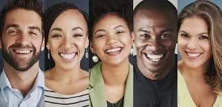
What happens when a human sees this image?
They will be able to recognize the face in the image. In simple terms, computer vision is about enabling computers to see and process visual data like humans. Computer vision involves analyzing images to produce useful information.
When you see an image of a mango, how do you recognize it as a mango?
By analyzing its color, shape, and texture, you can say it’s a mango.
The clues used to identify the image are called features of the image. Similarly, the function of computer vision is to detect various features in images.
We will discuss some algorithms in the OpenCV library used for feature detection.
1. Feature Detection Algorithms
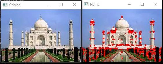
1.1 Harris Corner Detection
The Harris corner detection algorithm is used to detect corners in the input image. The algorithm has three main steps.
-
Determine which parts of the image have significant intensity changes since corners have large intensity changes. This is achieved by moving a sliding window across the entire image.
-
For each identified window, calculate a score R.
-
Apply a threshold to the scores and mark the corners.
This is the Python implementation of the algorithm.
import cv2
import numpy as np
imput_img = 'det_1.jpg'
ori = cv2.imread(imput_img)
image = cv2.imread(imput_img)
gray = cv2.cvtColor(image,cv2.COLOR_BGR2GRAY)
gray = np.float32(gray)
dst = cv2.cornerHarris(gray,2,3,0.04)
dst = cv2.dilate(dst,None)
image[dst>0.01*dst.max()]=[0,0,255]
cv2.imshow('Original',ori)
cv2.imshow('Harris',image)
if cv2.waitKey(0) & 0xff == 27:
    cv2.destroyAllWindows()
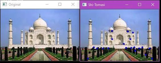
1.2 Shi-Tomasi Corner Detector
This is another corner detection algorithm. It works similarly to the Harris corner detection. The only difference here is the calculation of the R value. The algorithm also allows us to find the best n corners in the image.
Let’s look at the implementation in Python.
import numpy as np
import cv2
from matplotlib import pyplot as plt
img = cv2.imread('det_1.jpg')
ori = cv2.imread('det_1.jpg')
gray = cv2.cvtColor(img,cv2.COLOR_BGR2GRAY)
corners = cv2.goodFeaturesToTrack(gray,20,0.01,10)
corners = np.int0(corners)
for i in corners:
    x,y = i.ravel()
    cv2.circle(img,(x,y),3,255,-1)
cv2.imshow('Original', ori)
cv2.imshow('Shi-Tomasi', img)
cv2.waitKey(0)
cv2.destroyAllWindows()
This is the output of the Shi-Tomasi algorithm. Here, the top 20 corners are detected.
Next is the Scale-Invariant Feature Transform.
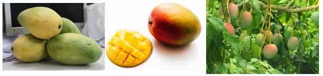
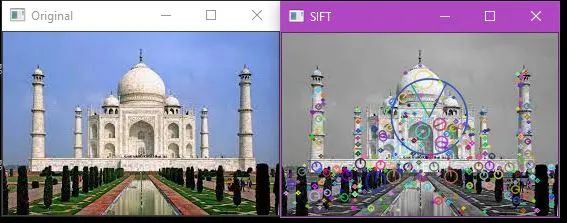
1.3 Scale-Invariant Feature Transform (SIFT)
SIFT is used to detect corners, blobs, circles, etc. It is also used for scaling images.
Consider these three images. Despite their differences in color, rotation, and angle, you know these are three different images of a mango. How can a computer recognize this?
In this case, both the Harris corner detection and Shi-Tomasi corner detection algorithms fail. But the SIFT algorithm plays a crucial role here. It can detect features from images regardless of their size and orientation.
Let’s implement this algorithm.
import numpy as np
import cv2 as cv
ori = cv.imread('det_1.jpg')
img = cv.imread('det_1.jpg')
gray = cv.cvtColor(img,cv.COLOR_BGR2GRAY)
sift = cv.SIFT_create()
kp, des = sift.detectAndCompute(gray,None)
img=cv.drawKeypoints(gray,kp,img,flags=cv.DRAW_MATCHES_FLAGS_DRAW_RICH_KEYPOINTS)
cv.imshow('Original',ori)
cv.imshow('SIFT',image)
if cv.waitKey(0) & 0xff == 27:
    cv.destroyAllWindows()
The output is shown below.
You can see some lines and circles in the image. The size and orientation of the features are represented by circles and lines within the circles, respectively.
We will see the next feature detection algorithm.
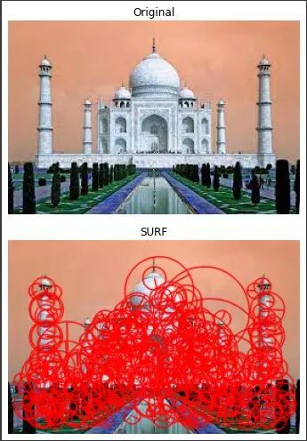
1.4 Speeded-Up Robust Features (SURF)
The SURF algorithm is simply an upgrade of SIFT.
Here is the code implementation:
import numpy as np
import cv2 as cv
ori =cv.imread('/content/det1.jpg')
img = cv.imread('/content/det1.jpg')
surf = cv.xfeatures2d.SURF_create(400)
kp, des = surf.detectAndCompute(img,None)
img2 = cv.drawKeypoints(img,kp,None,(255,0,0),4)
cv.imshow('Original', ori)
cv.imshow('SURF', img2)
Next, we will see how to extract another feature called BLOB.
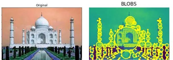
2. BLOB Detection
BLOB stands for Binary Large Object. It refers to a set of connected pixels or regions in a specific binary image that share common properties. These regions are contours in OpenCV, with some additional features like centroid, color, area, mean, and standard deviation of pixel values in the coverage area.
Here is the code implementation:
import cv2
import numpy as np;
ori = cv2.imread('det_1.jpg')
im = cv2.imread("det_1.jpg", cv2.IMREAD_GRAYSCALE)
detector = cv2.SimpleBlobDetector_create()
keypoints = detector.detect(im)
im_with_keypoints = cv2.drawKeypoints(im, keypoints, np.array([]), (0,0,255), cv2.DRAW_MATCHES_FLAGS_DRAW_RICH_KEYPOINTS)
cv2.imshow('Original',ori)
cv2.imshow('BLOB',im_with_keypoints)
if cv2.waitKey(0) & 0xff == 27:
    cv2.destroyAllWindows()
Let’s look at the output. Here, the BLOBs are well detected.
Now, let’s move on to feature descriptor algorithms.
3. Feature Descriptor Algorithms
Features are typically different points in an image, and descriptors give the features, thus describing the key points in consideration. It extracts the local neighborhood around that point, creating local image patches and calculating features from that local patch.
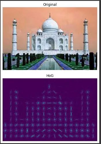
3.1 Histogram of Oriented Gradients (HoG)
Before the advent of deep learning, HoG was one of the most prominent feature descriptors in object detection applications. HoG is a technique used to compute the occurrence of gradient directions in the local image.
Let’s implement this algorithm.
from skimage.feature import hog
import cv2
ori = cv2.imread('/content/det1.jpg')
img = cv2.imread("/content/det1.jpg")
_, hog_image = hog(img, orientations=8, pixels_per_cell=(16, 16),
                    cells_per_block=(1, 1), visualize=True, multichannel=True)
cv2.imshow('Original', ori)
cv2.imshow('HoG', hog_image)
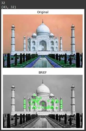
3.2 Binary Robust Invariant Scalable Keypoints (BRIEF)
BRIEF is an alternative to the popular SIFT descriptor, which computes faster and is more compact.
Let’s look at its implementation.
import numpy as np
import cv2 as cv
ori = cv.imread('/content/det1.jpg')
img = cv.imread('/content/det1.jpg',0)
star = cv.xfeatures2d.StarDetector_create()
brief = cv.xfeatures2d.BriefDescriptorExtractor_create()
kp = star.detect(img,None)
kp, des = brief.compute(img, kp)
print( brief.descriptorSize() )
print( des.shape )
img2 = cv.drawKeypoints(img, kp, None, color=(0, 255, 0), flags=0)
cv.imshow('Original', ori)
cv.imshow('BRIEF', img2)
3.3 Oriented FAST and Rotated BRIEF (ORB)
ORB is a one-time facial recognition algorithm. It is currently used in apps like Google Photos, where you can group people based on the images you see.
This algorithm does not require any major computation. It does not need a GPU. It’s fast and concise. It’s suitable for matching key points in different areas of the image, such as intensity changes.
Below is the implementation of this algorithm.
import numpy as np
import cv2
ori = cv2.imread('/content/det1.jpg')
img = cv2.imread('/content/det1.jpg', 0)
orb = cv2.ORB_create(nfeatures=200)
kp = orb.detect(img, None)
kp, des = orb.compute(img, kp)
img2 = cv2.drawKeypoints(img, kp, None, color=(0, 255, 0), flags=0)
cv2.imshow('Original', ori)
cv2.imshow('ORB', img2)
Now, let’s look at feature matching.
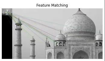
4. Feature Matching
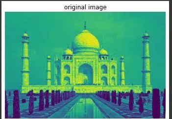
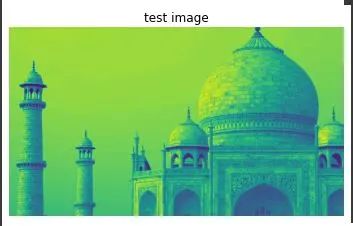
Feature matching is like comparing features of two images that may differ in direction, perspective, brightness, and even size and color. Let’s look at its implementation.
import cv2
img1 = cv2.imread('/content/det1.jpg', 0)
img2 = cv2.imread('/content/88.jpg', 0)
orb = cv2.ORB_create(nfeatures=500)
kp1, des1 = orb.detectAndCompute(img1, None)
kp2, des2 = orb.detectAndCompute(img2, None)
bf = cv2.BFMatcher(cv2.NORM_HAMMING, crossCheck=True)
matches = bf.match(des1, des2)
matches = sorted(matches, key=lambda x: x.distance)
match_img = cv2.drawMatches(img1, kp1, img2, kp2, matches[:50], None)
cv2.imshow('original image', img1)
cv2.imshow('test image', img2)
cv2.imshow('Matches', match_img)
cv2.waitKey()
This is the result of this algorithm.
Conclusion
I hope you enjoyed this article. I have briefly introduced various feature detection, description, and matching techniques. The above techniques are used in object detection, object tracking, and object classification applications.
The real fun begins when you start practicing. So, start practicing these algorithms, implement them in real projects, and see the fun in it. Keep learning.
Download 1: OpenCV-Contrib Extension Module Chinese Version Tutorial

Reply 'Extension Module Chinese Tutorial' in the backend of 'Xiaobai Learns Vision' public account to download the first Chinese version of the OpenCV extension module tutorial, covering installation of extension modules, SFM algorithms, stereo vision, object tracking, biological vision, super-resolution processing, and more than twenty chapters of content.

Download 2: Python Vision Practical Projects 52 Lectures

Reply 'Python Vision Practical Projects' in the backend of 'Xiaobai Learns Vision' public account to download 31 practical vision projects, including image segmentation, mask detection, lane line detection, vehicle counting, adding eyeliner, license plate recognition, character recognition, emotion detection, text content extraction, facial recognition, etc. to help quickly learn computer vision.

Download 3: OpenCV Practical Projects 20 Lectures

Reply 'OpenCV Practical Projects 20 Lectures' in the backend of 'Xiaobai Learns Vision' public account to download 20 practical projects based on OpenCV to achieve advanced learning of OpenCV.

Discussion Group

Welcome to join the reader group of the public account to communicate with peers. Currently, there are WeChat groups for SLAM, 3D vision, sensors, autonomous driving, computational photography, detection, segmentation, recognition, medical imaging, GAN, algorithm competitions, etc. (which will gradually be subdivided in the future). Please scan the following WeChat number to join the group, and note: 'Nickname + School/Company + Research Direction', for example: 'Zhang San + Shanghai Jiaotong University + Visual SLAM'. Please follow the format for notes, otherwise, it will not be passed. After successful addition, you will be invited to enter the relevant WeChat group according to your research direction. Please do not send advertisements in the group, otherwise, you will be removed. Thank you for your understanding~