

Star★TopPublic Account I love you all♥
0
Introduction
Today, the public account will introduce to everyone,distinguishing real financial time series from synthetic time series. The data is anonymous, and we do not know which time series comes from which asset.
In the end, we achieved a 67% in-sample testing accuracy and a 65% out-of-sample testing accuracy.
We have 12,000 real time series and 12,000 synthetic created time series, totaling 24,000 observations.
The full text is divided into three parts, let’s start,very interesting!
1
Preparation Work
Import related libraries:
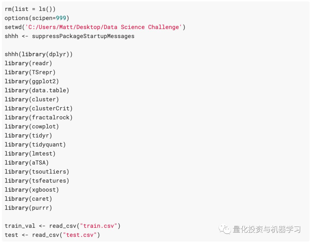
Note: We have two datasets, train_Val.csv for training and validation data, and test.csv dataset. I only touch the test.csv dataset at the end of part 3. All analysis and optimization are performed only on the train_val.csv dataset. train_val.csv contains 12,000 observations, and test.csv contains 12,000 observations.
2
First Part
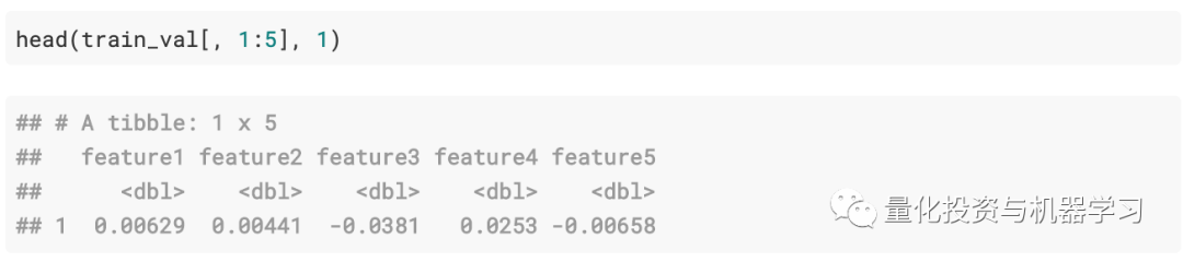
Data Format:
The column names are as follows:
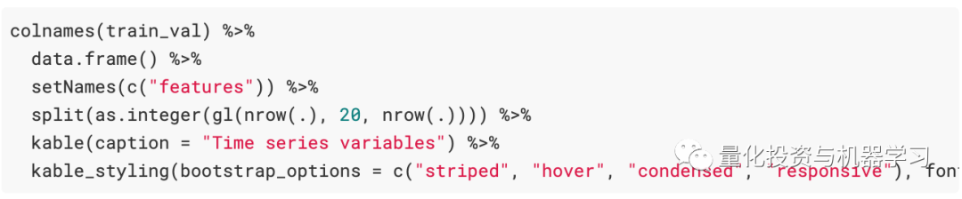
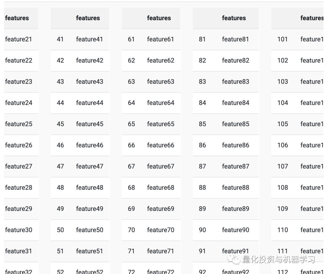
The training data has 260 “features” and a categorical variable excluded from the test data. There are about 253 trading days in a year, feature1, feature2, … featureN are daily time series. From the initial observations (and plots), we consider the data to be “returns” data. First, to clean some data, since the time series performs poorly when using feature1, feature2, … featureN as inputs. We randomly select a year and use the function getTradingDates to rename these columns (there’s always a universal R package…).
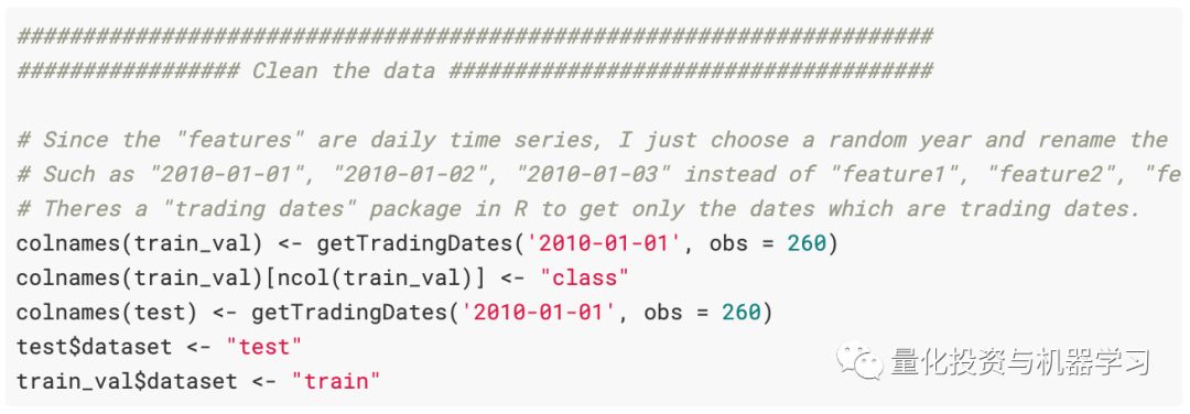
Here (if we do something different), we will maintain the tidy data principle and use test %>% add_column(dataset = “test”) and train %>% add_column(dataset = “train”) instead of test$dataset <- “test” and train_val$dataset <- “train”. But that’s okay.
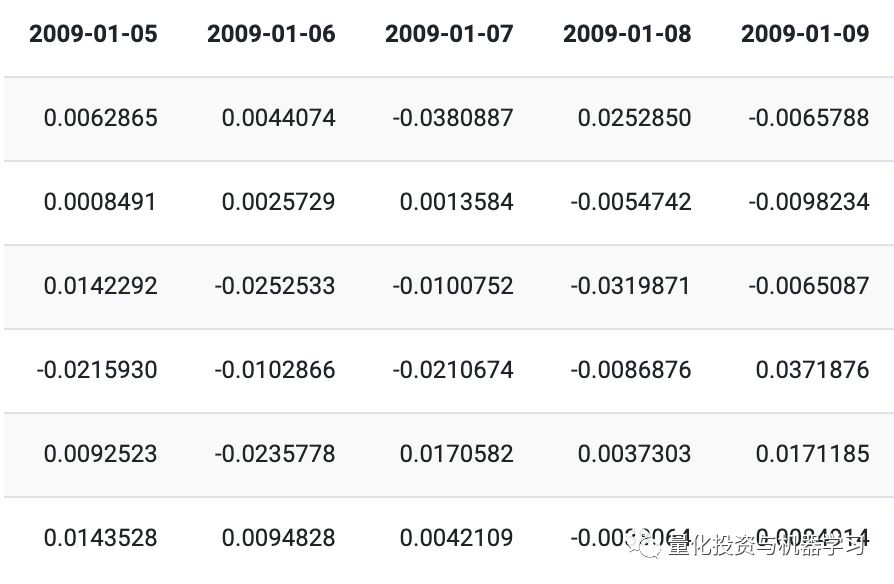
Cleaned training data:
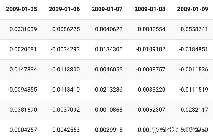
Cleaned test data:
Objective: The goal is to classify which financial time series are real and which are synthetically created (by some algorithm, we do not know how the synthetic time series are generated).
We rearranged the data using the melt function in R, but it is recommended that anyone reading this document use the pivot_longer function from the tidyverse package. You can refer to the pivot_longer package.

Note: We refer to the training data as df, which in hindsight is a bad practice; it should be named something related to the train_Val dataset. Remember, df refers to the train_Val dataset. (And does not include data from the test.csv dataset)
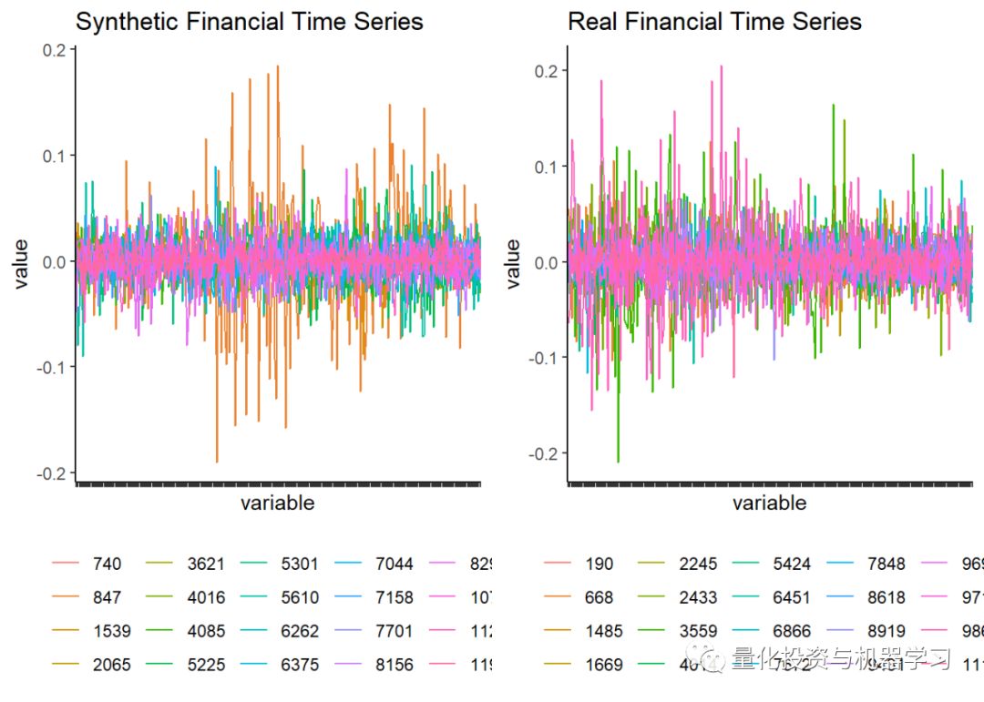
As we see, the data has 3,120,000 rows, which is 12,000 assets * 260 trading days. Next, we use ggplot to plot the return series.
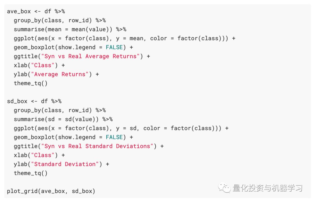
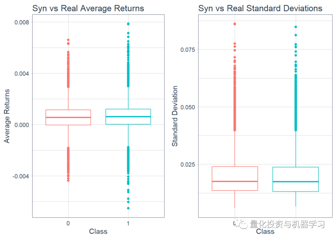
Next, we plot boxplots to get the average return rates, followed by the standard deviations.
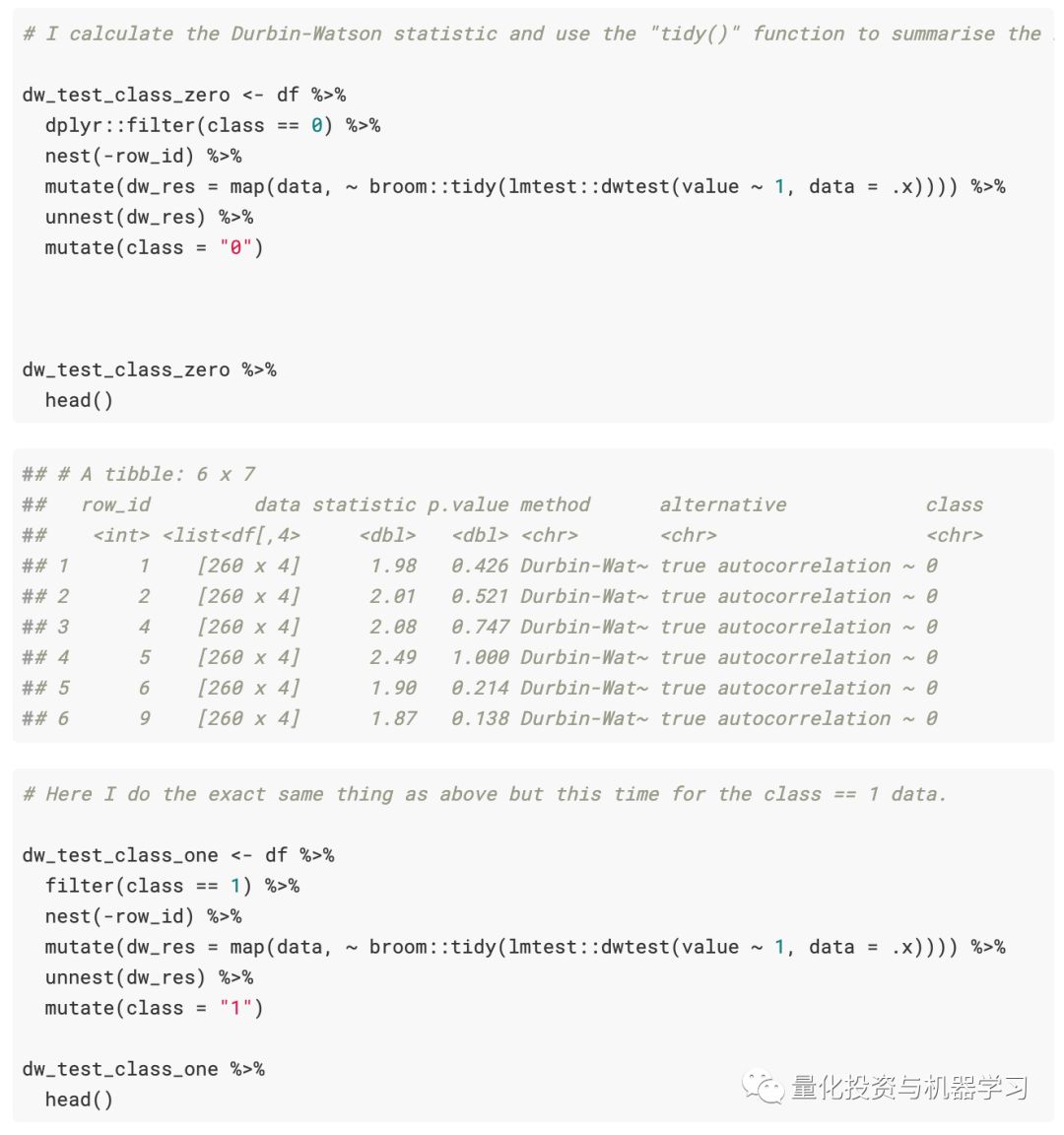
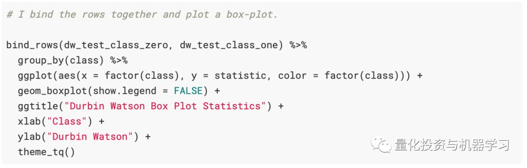
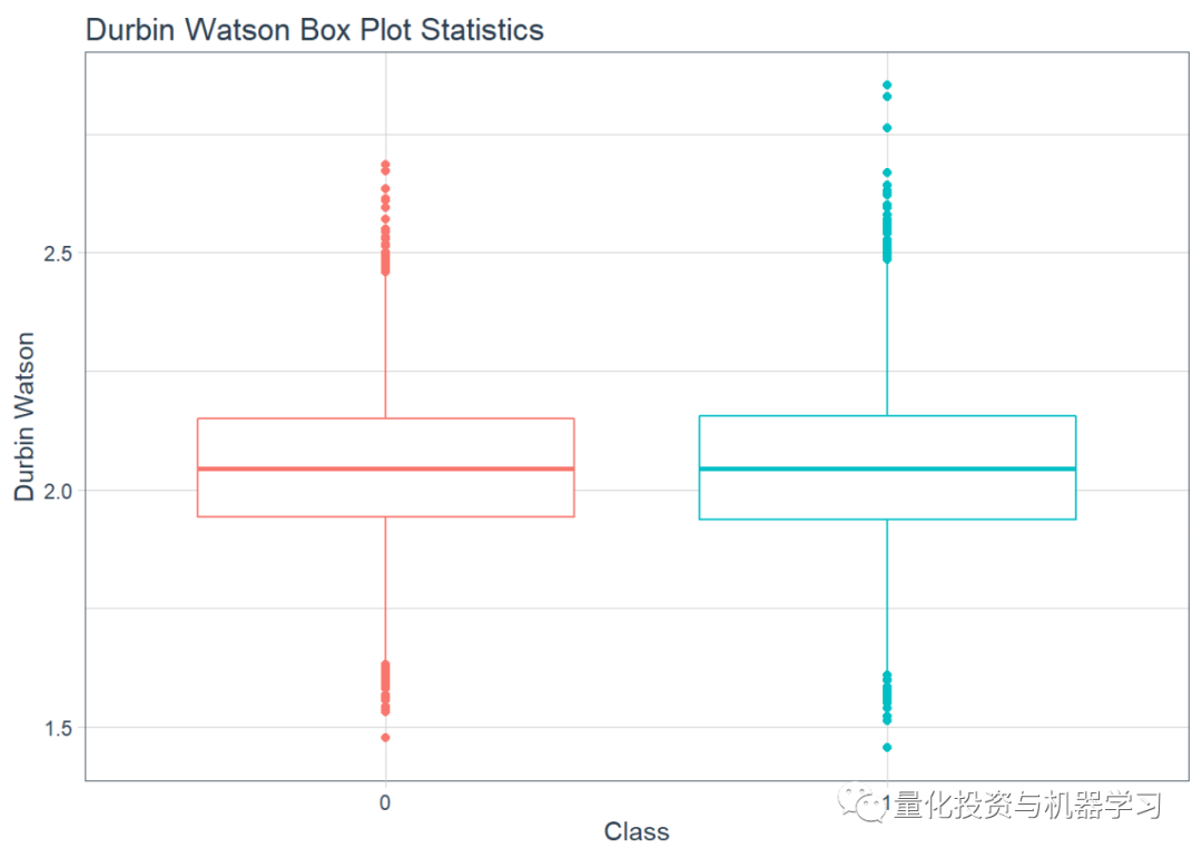
Next, we calculate the Durbin-Watson statistics. The main coding is done using the tidy data principles in R, so we use the tidy function from the broom package to slightly tidy up the output of the DW statistics. This is done for both synthetic and real time series.
Next, we plot boxplots of the Durbin-Watson test statistics for each.
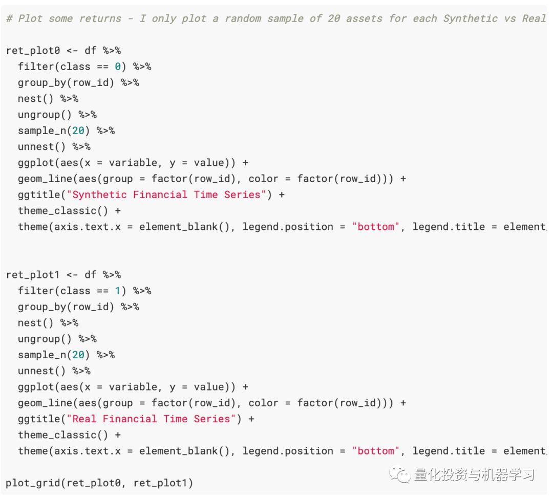
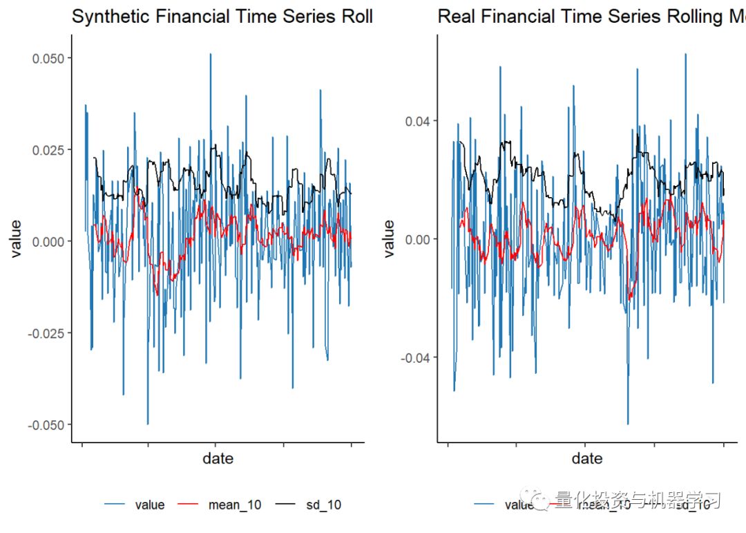
Using the tq_mutate function from the tidyquant package, we calculated the 10-day rolling mean and standard deviation. The value corresponds to the returns of the financial time series, plotted in blue, with the 10-day rolling mean and standard deviation drawn on the returns. (Again, we used melt here, but checked the pivot_longer function for a more intuitive application)
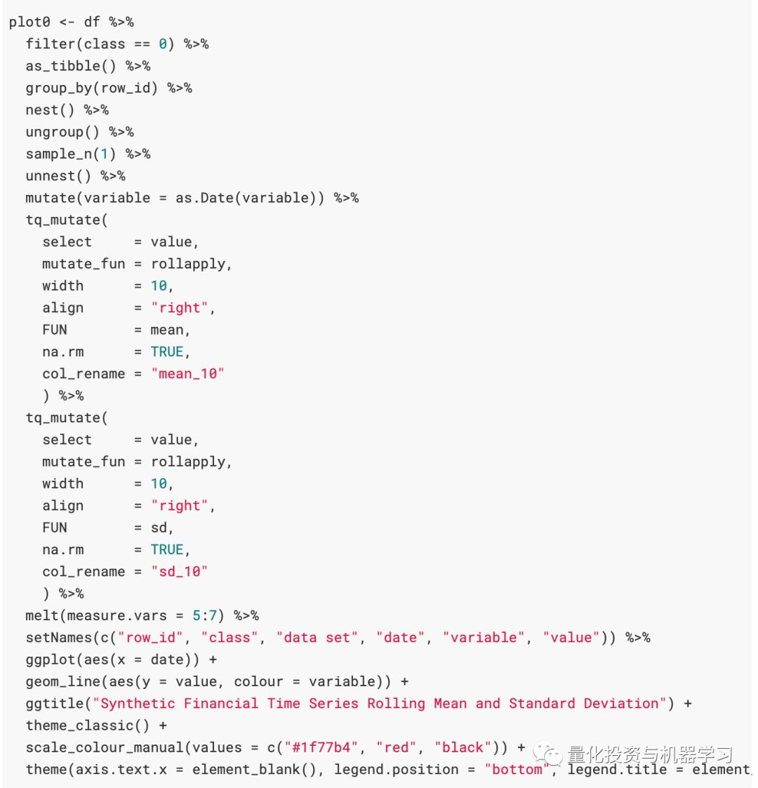

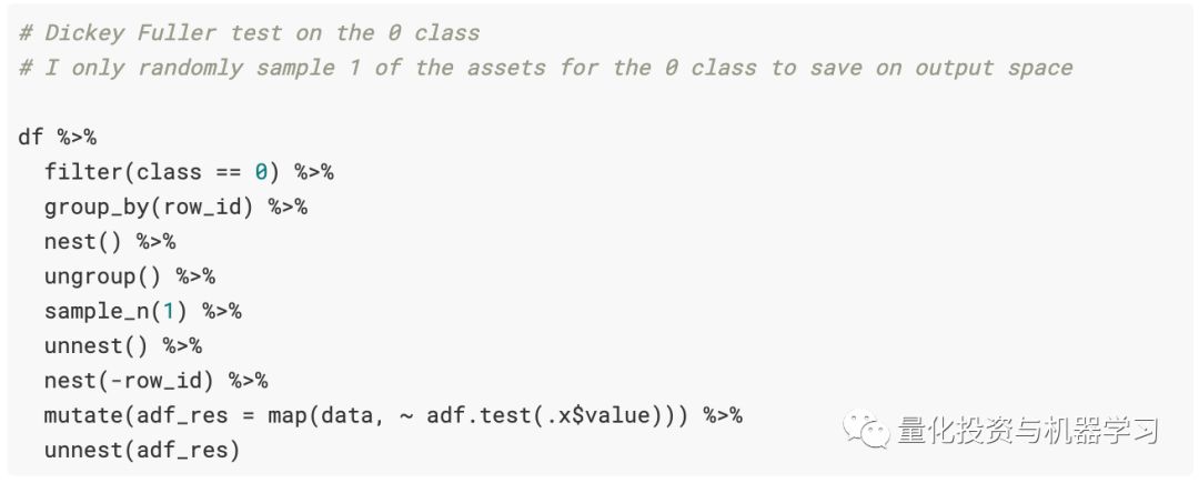
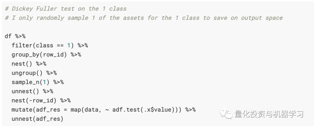
An important note in the code here is that we are sampling by group, meaning we do not randomly sample from all observations across all groups. Instead, we group each time series (filtering on class == 0 for each of the 6,000 observations, and similarly for class == 1), and then nest() the daily time series of each asset into a list. From here we will have 6,000 observations, each with its time series nested within the list. Therefore, we can sample one of the 6,000 observations and then unnest() to get the full time series set of one of the randomly selected assets, rather than randomly sampling from the time series data of all assets (which would be completely wrong).
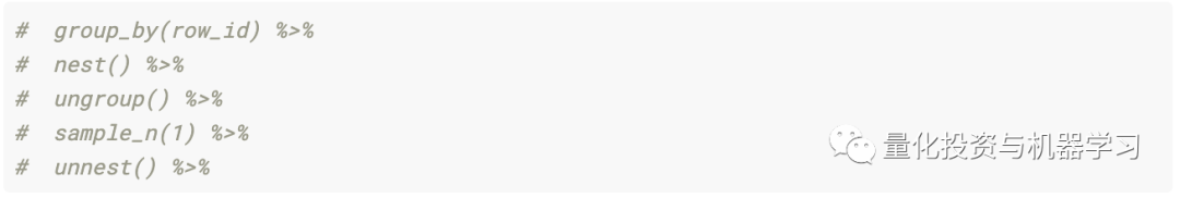
For example, the commented code below requires the ID variable in group_by() and the data in nest(), needing a random sample_n() from the grouped data, and then unnest() the data back to its original form, using the random sample IDs.
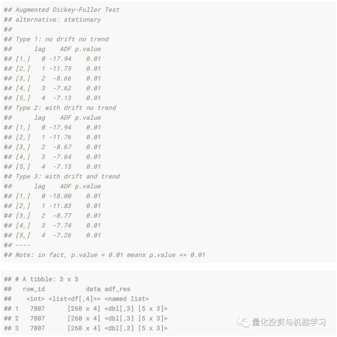
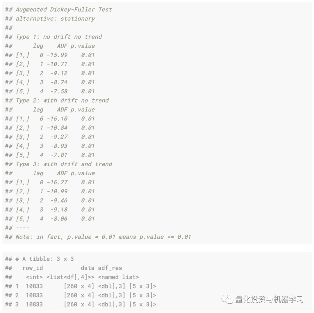
Next, we calculate the Dickey-Fuller test for a random observation on the two sequences, thus calculating the sample_n(1) parameter (to calculate on all 12,000 observations is very expensive).
Syntheticsequence:
Real financial sequence:
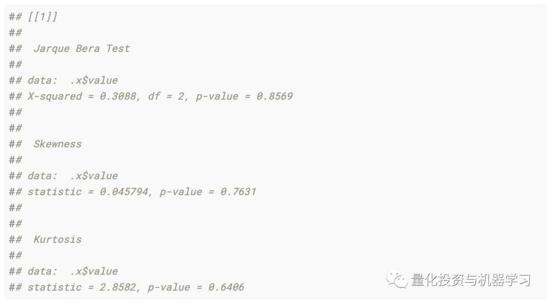
Next is the Jarque-Bera normality test. First for the synthetic sequence:

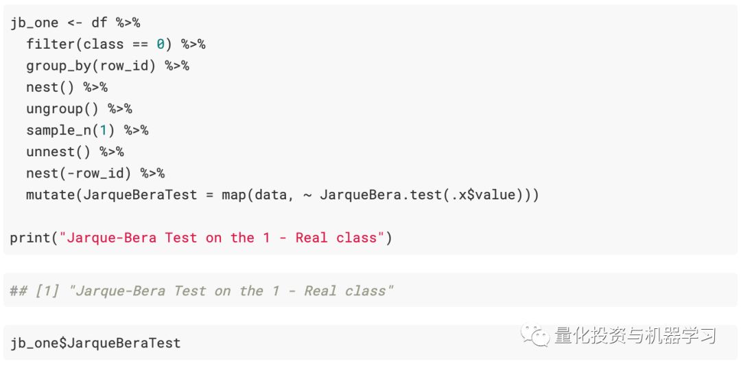
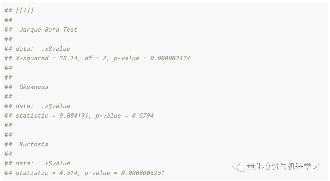
Real financial sequence:
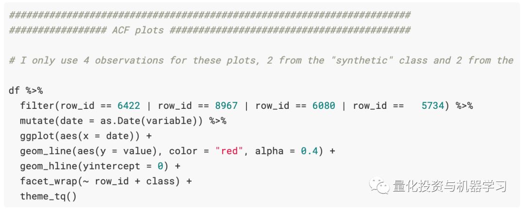
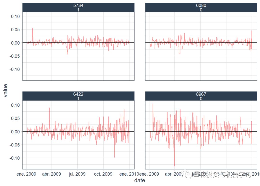
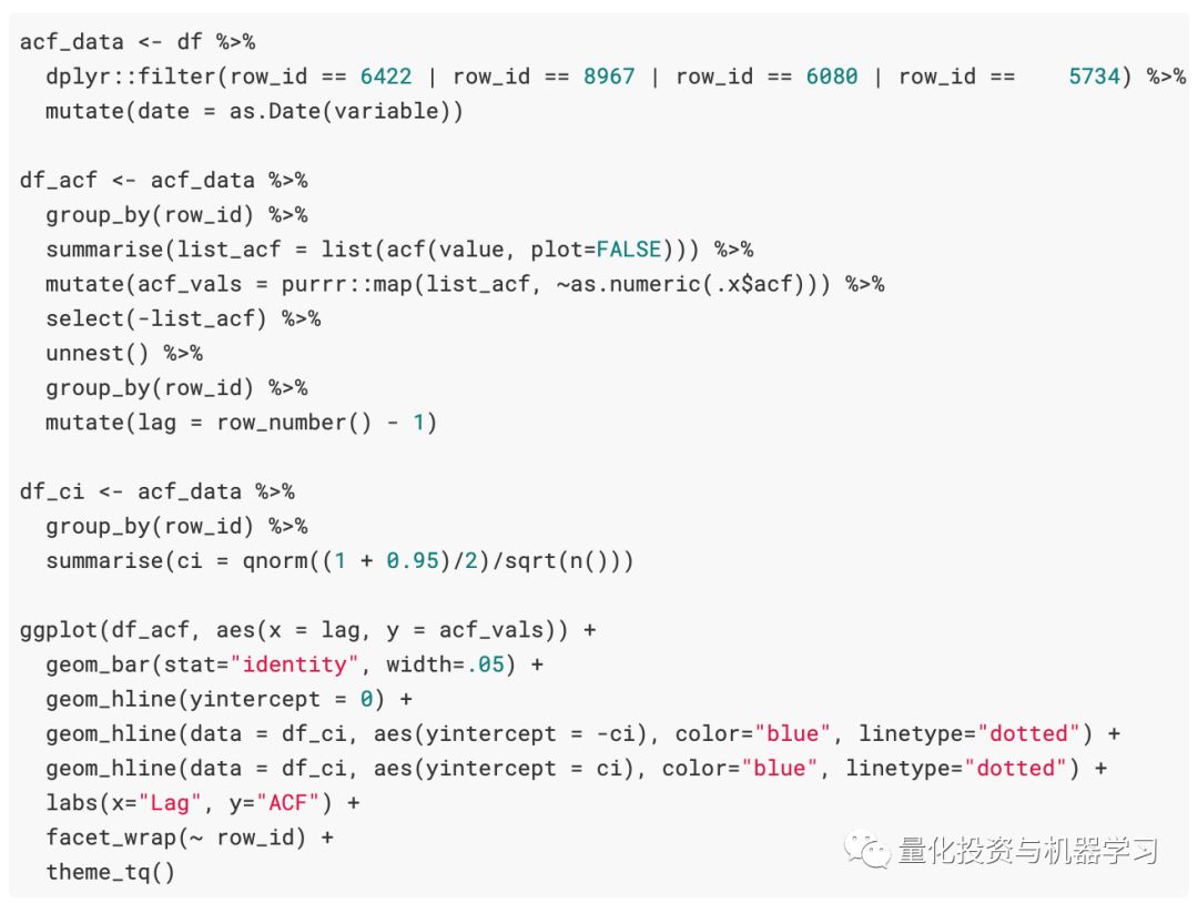
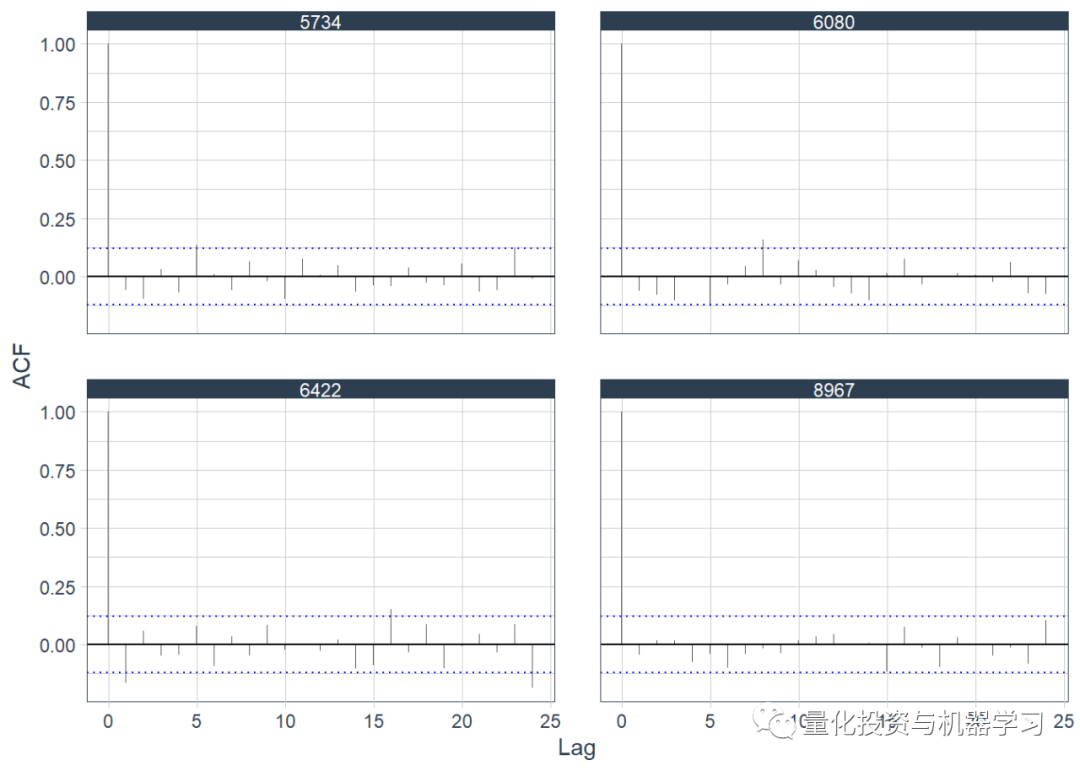
Autocorrelation Plot
A “random” sample of the observed time series was plotted for the autocorrelation function. We selected 4 observations and filtered the data based on them.
With sufficient data analysis, we might also simultaneously conduct PACF plots and some other exploratory data analysis, continuing to generate financial time series features using the tsfeatures package.
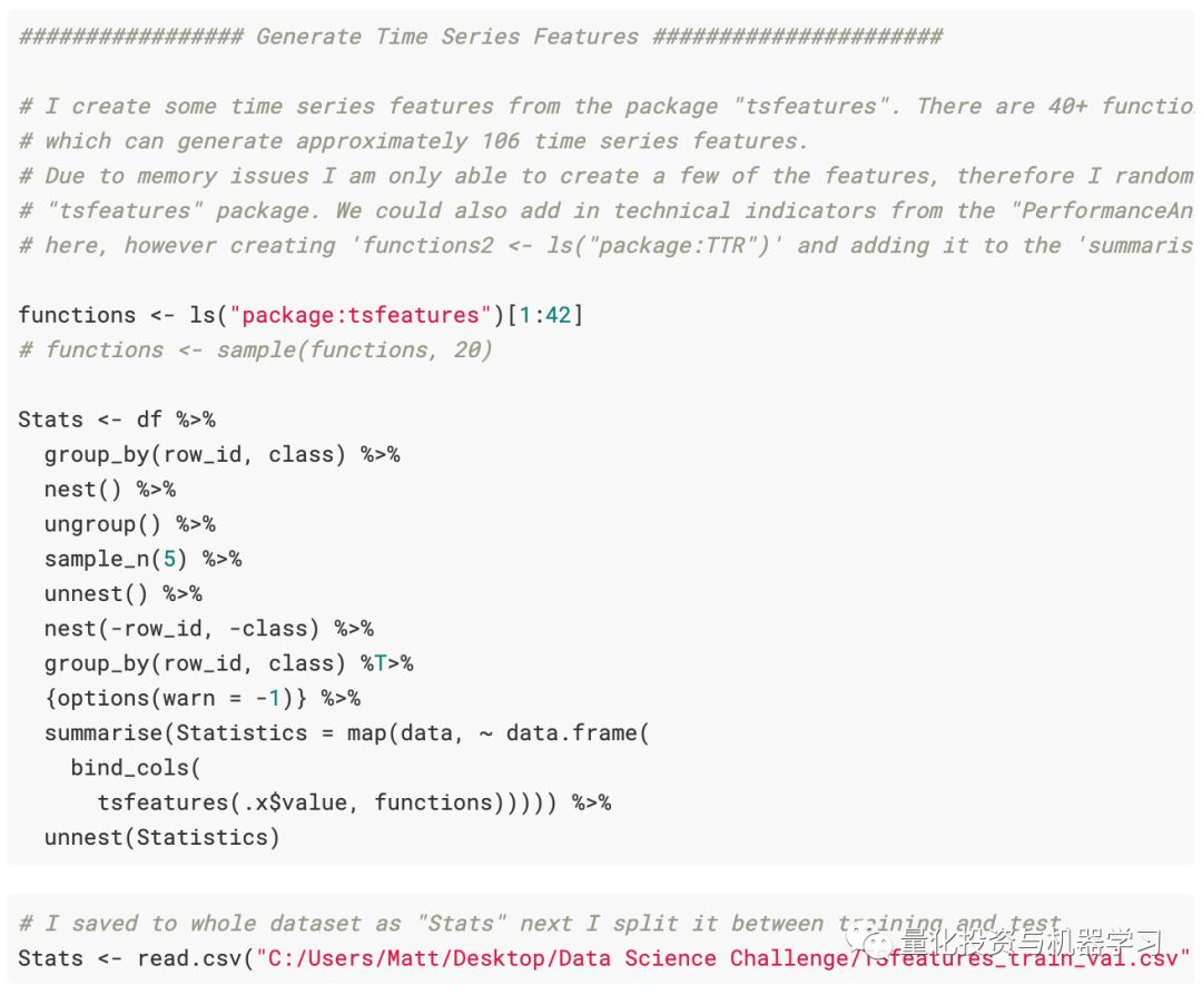
What is done in the code below is to randomly sample 5 groups (it takes a long time to calculate time series features using the entire dataset), and then apply all functions from the tsfeatures package to each time series asset data by mapping each asset data and calculating time series features.
3
Second Part
This section requires some time to process and calculate (especially on the entire sample), we have saved the results as csv, I will use it and load it into the pre-calculated time series features.
Note: The wrong practice is simply calling the df data Stats, which only contains time series features data. This still only references the train_val.csv data, not the test.csv data.
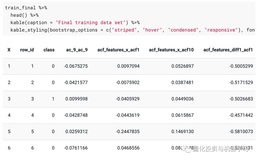
The training data looks like: (after calculating the time series features). Now, each asset has been decomposed from about 260 days into one signal time series feature observation.
Recall that the goal here is to classify synthetic time series from real time series, not the price the next day. For each asset, we have a signal observation, based on which we can train a classification algorithm to distinguish real time series from synthetic time series.
Training Data:
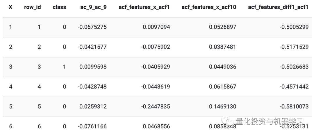
The size of the data is still 12,000, with 109 features (created from the tsfeatures package). That is, we have 6,000 synthetic and 6,000 real financial time series (12,000 * ~260 = 3,120,000, but we apply tsfeatures to decompose each asset’s ~260 into one single observation)
We have broken down this problem from a time series forecasting problem into a pure classification problem. Next, we split the data between the training and validation sets… we will also split the data into X_train, Y_train … etc.
Split the df / Stats dataset into a training set of 75% of observations and a sample in-test dataset of 25% of observations.
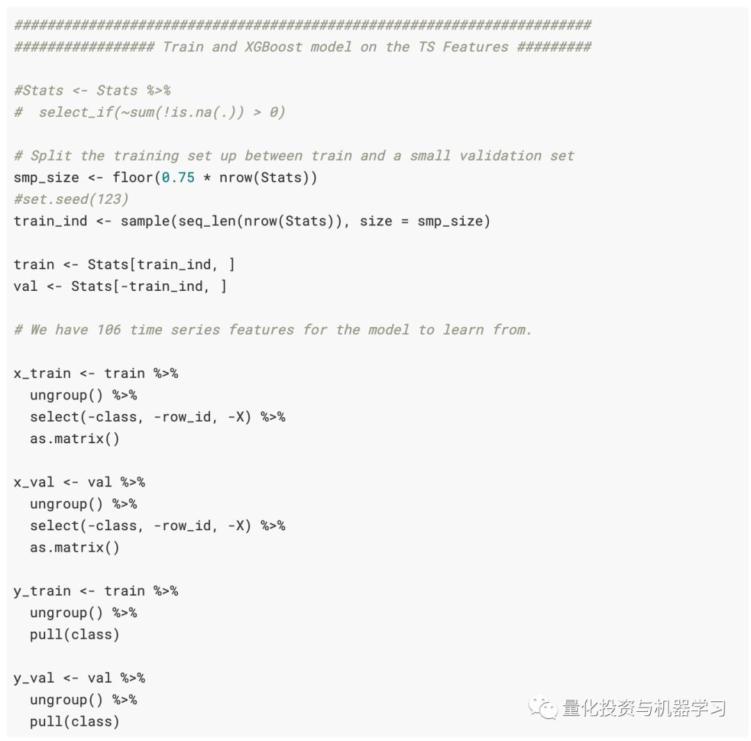
Training X (input variable) data:
Training Y (predictive variable) data:
We set up the data for the XGBoost model:
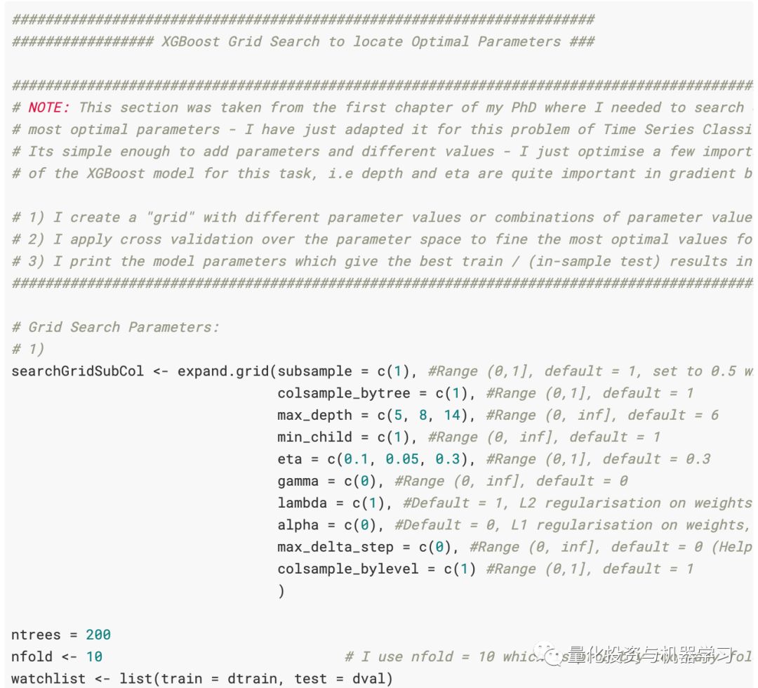
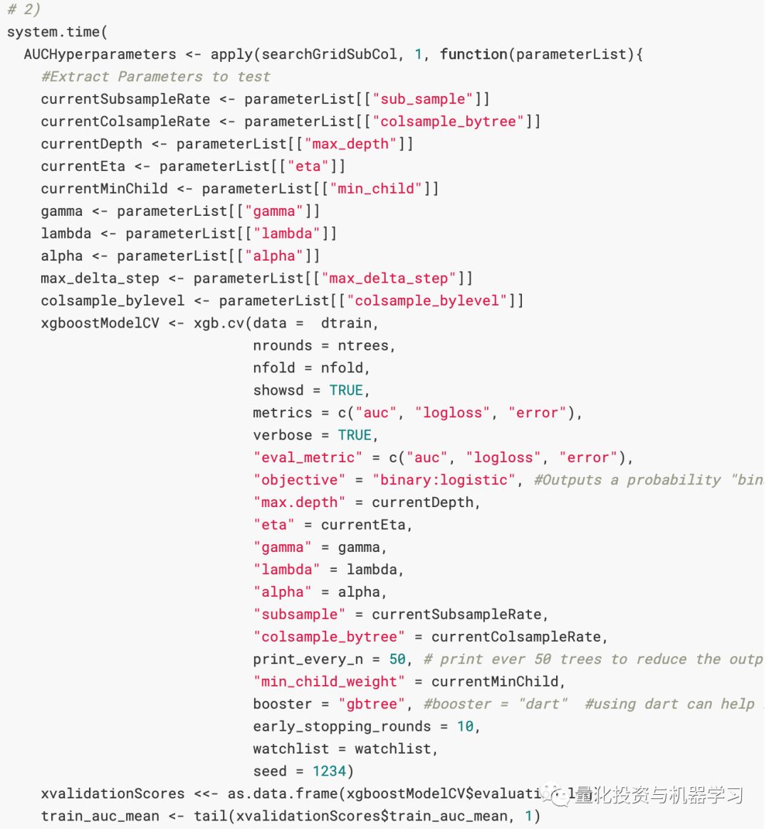
A grid search was created to search the parameter space to find the best parameters for the dataset. More work needs to be done, but this is a good starting point. Code can be added to the expand.grid function. That is, for example, if we want to increase the depth of the tree, we can add more parameters to max_depth = c(5, 8, 14), such as max_depth = c(5, 8, 14, 1, 2, 3, 4, 6, 7). Note that adding parameters to the grid search will exponentially increase computation time. You add a value to each parameter, and the model must search all possible combinations associated with that parameter. That is, adding eta = c(0.1) and max_depth = c(5) will provide us with the best parameters for one iteration/cycle in training the model, i.e., mapping eta = c(0.1) to max_depth = c(5). Adding an additional value, such as eta = c(0.1, 0.3) and max_depth = c(5) will map eta = 0.1 to max_depth = 5 and eta = 0.3 to max_depth = 5. If I add another value, like eta = c(0.1, 0.3, 0.4), all three values will map to max_depth = c(5). Adding values to the max_depth = c(5) parameter will add an extra layer of complexity to the grid search. There are many parameters to optimize in the XGBoost model, which significantly increases computational complexity. Therefore, when trying to avoid getting stuck in local minima (any greedy algorithm using gradient descent optimization can do this: greedy algorithms), it is very important to understand the statistics behind the models in machine learning.
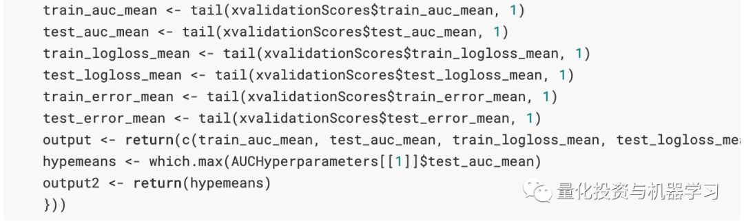
The output of the grid search can be set to a nice data frame using the following code. However, we did not save this output to a file, so we cannot read it.
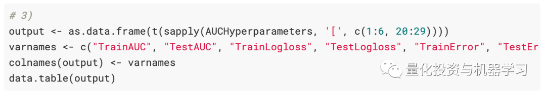
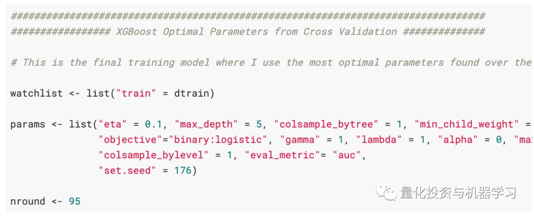
Based on the results at the time, the best parameters were:
-
ntrees = 95,
-
eta = 0.1,
-
max_depth = 5
For simplicity, the other parameters are kept at their default settings.
4
Third Part
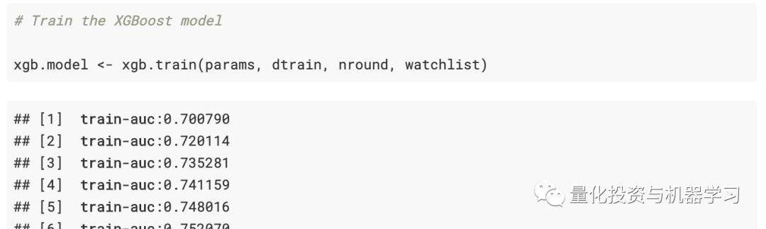
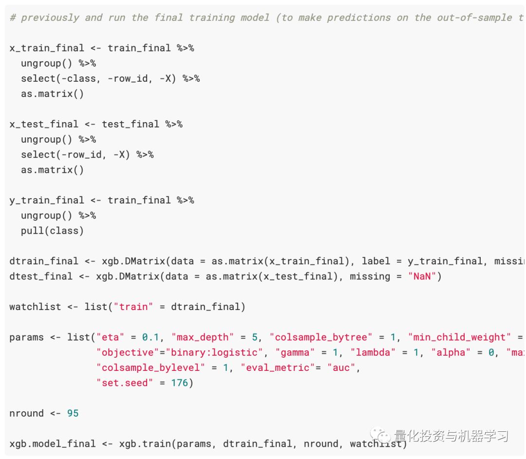
Now, we have obtained the best parameters from the cross-validation grid search and can train the final XGBoost model on the entire train_val.csv dataset.
The advantage of tree-based models is that we can obtain importance scores from the model and find out which variables contribute the most to the model’s returns.
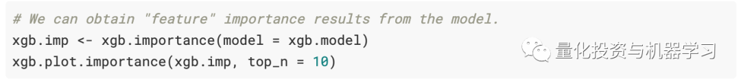
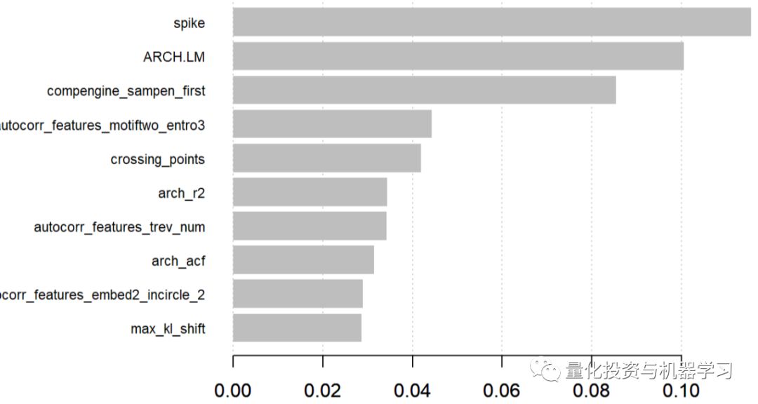
That is, the XGBoost model found that the spike is the most important variable. The spike comes from the stl_features function of the tsfeatures package in R. It calculates various measures of trend and seasonality based on seasonal and trend decomposition (STL) and measures the spikiness of the time series based on the variance of the component e_t.
The second variable is also interesting, it comes from the compenginefeature set of the CompEngine database. It groups variables into autocorrelation, prediction, stationarity, distribution, and scaling.
ARCH.LM comes from the arch_stat function of the tsfeatures package and is based on autoregressive conditional heteroskedasticity (ARCH) Engle1982’s Lagrange multiplier.
These are just a few of the most important variables found by the XGBoost model. A complete overview and more information on the variables used in the model can be found here.
Predicting Using the In-Sample Test Set
Now that we have trained the model with the best parameters, we want to see if its score is the same or higher based on the validation data from the cross-validation phase. We use dval (which is the validation dataset from the training group) to validate the model.
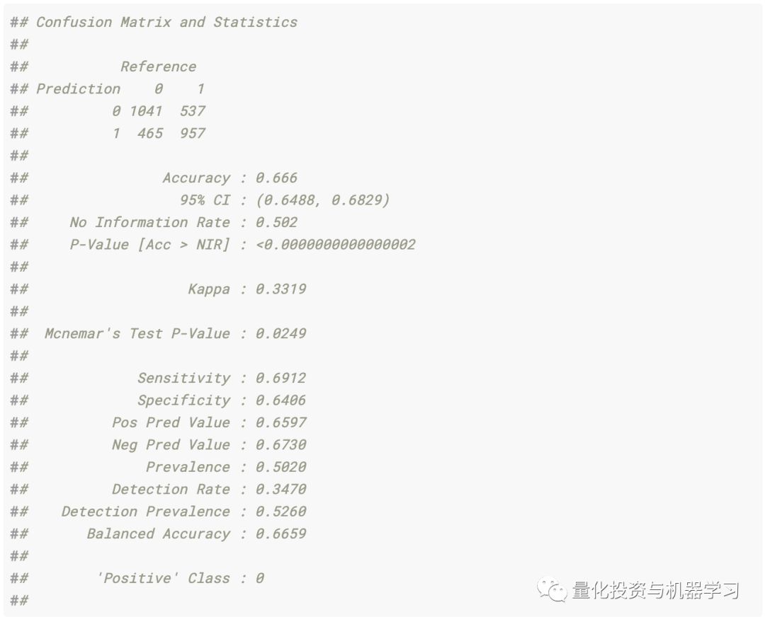
This is a time series (stock market) classification problem, so a balanced accuracy score of 67% is not bad.
From here we conclude the training and validation of the model. We have obtained the best values based on the training and validation datasets, and now we want to test it on the unknown data test.csv.
The test data was read, and the time series features were calculated from the tsfeatures package, just like the training data was processed.
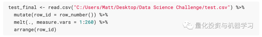
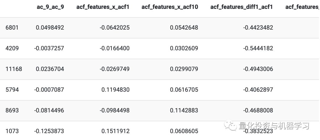
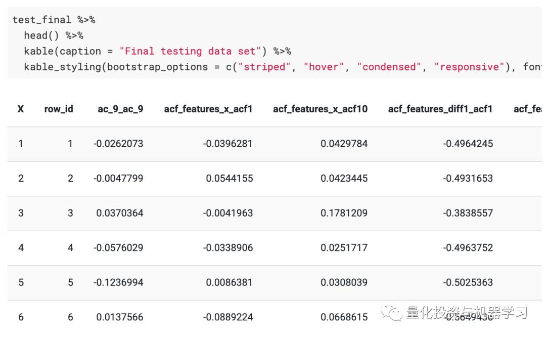
The appearance of the test features (they look similar to the training dataset):
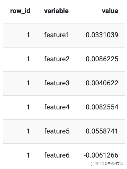
We call it test_final, and for no reason we test it – it has been the same test.csv from the beginning.
Next, we create the same time series features on the test dataset as we did on the training dataset. Save it as TSfeatures_test.csv.
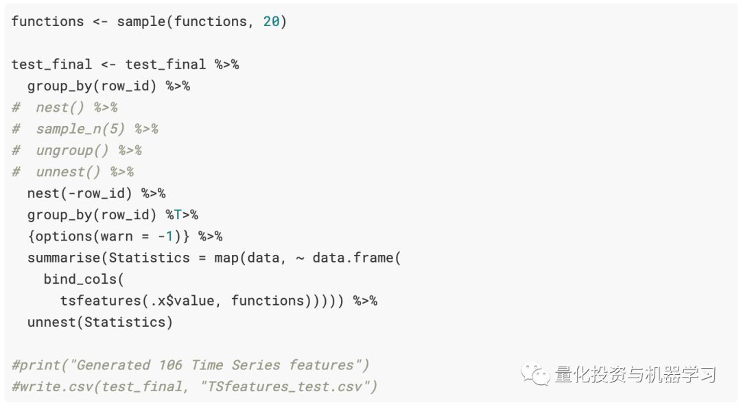
We have calculated all tsfeatures for both the training and test datasets. Save these as TSfeatures_train_val.csv and TSfeatures_test.csv.
Loading the Training and Testing Feature Datasets
The final data for training and testing are as follows:
Finally, we can run the final model on the held-out test set and get our predictions based on the training data and the best parameters.
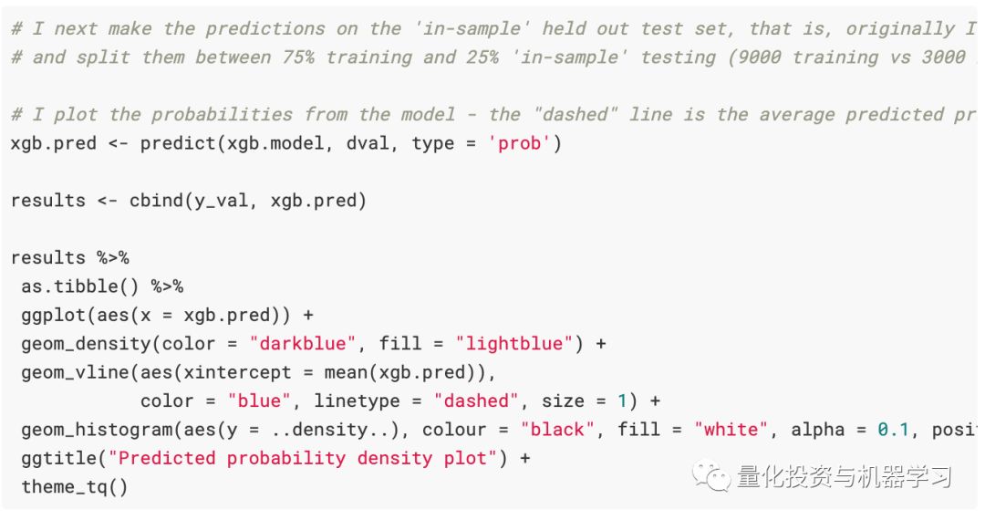
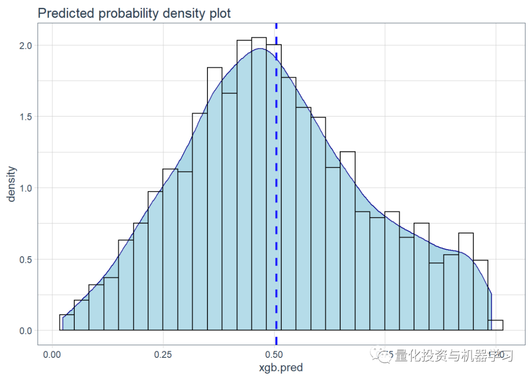
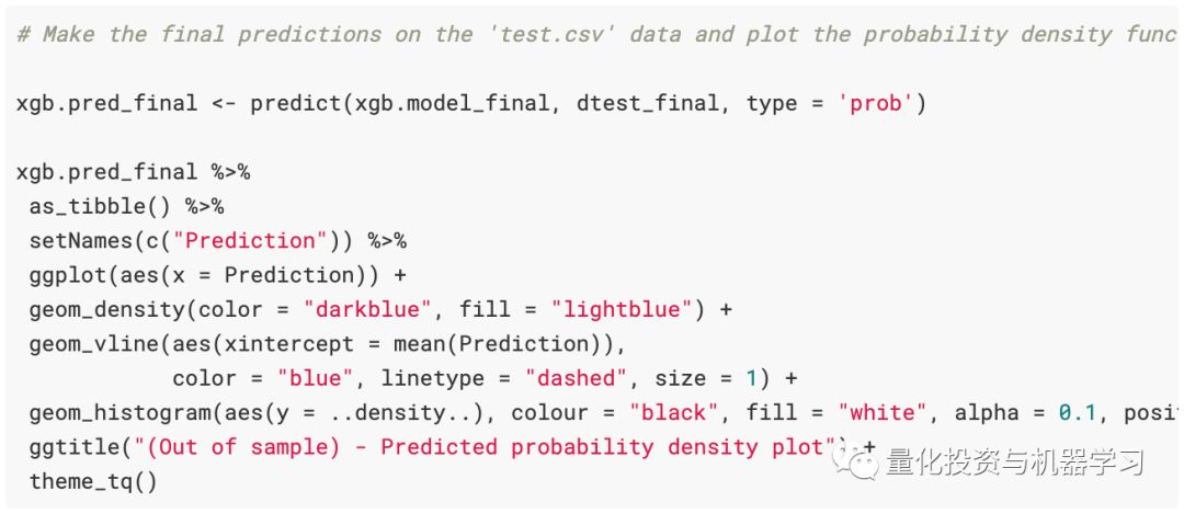
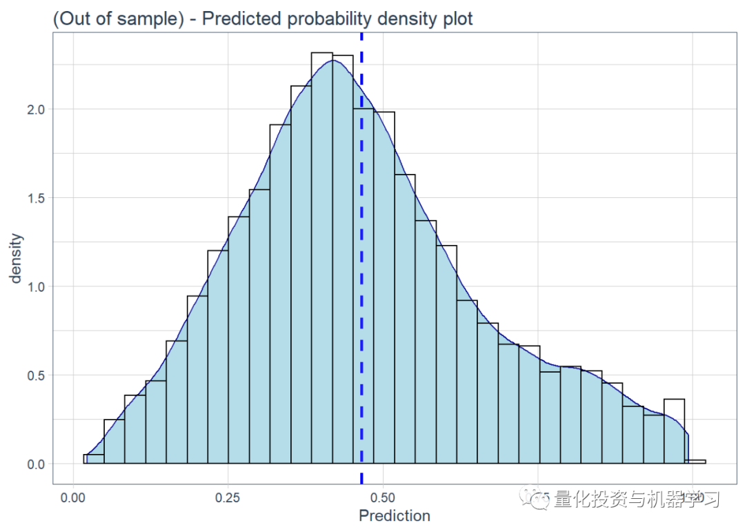
Based on the test.csv data, we make the final predictions. The predict function in R is great; it can take any model for prediction, and we just need to provide the test data along with the model. We also plotted the density of the predicted probabilities.
Finally! Submit the file based on the predicted probabilities.
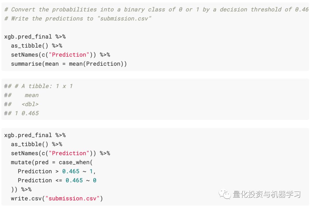
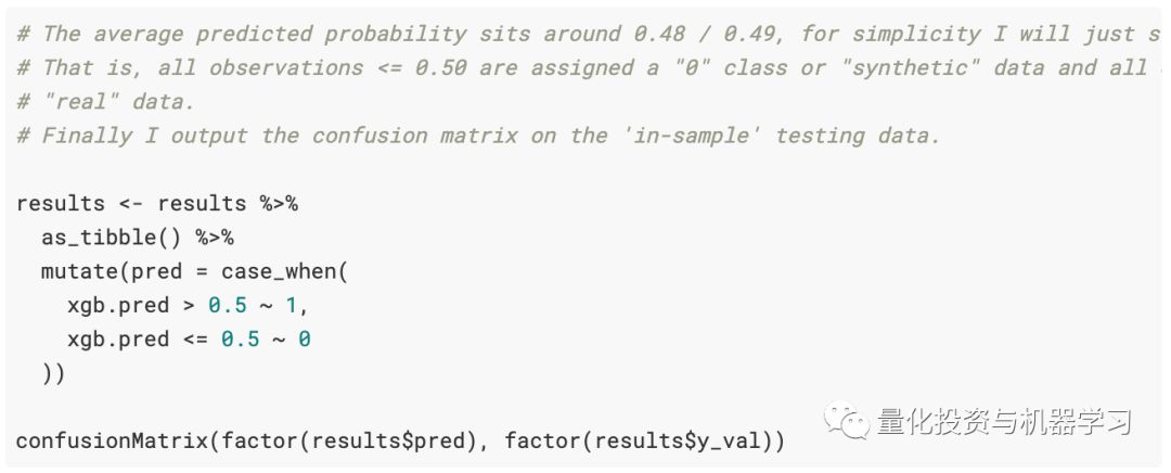
How to evaluate scores:
Results between 0.4-0.6 are considered random results.
Starting from 0.6, the algorithm correctly classifies, and algorithms above 0.7 are great.
Below 0.4, they can distinguish between synthetic sequences and real-time sequences, but they are interchangeable.
Based on the held-out test set, we obtained results of 0.649636 ~ 0.65% (which is slightly lower than the 0.67% in-sample training set!), but still consistent with the correct method we used (i.e., no leakage of test data into the training data).
5
Summary
The combination of time series feature selection and classification models can handle the time series classification problem we are facing very well!
Everyone keep it up!
Concerned about Wuhan
The mountains and rivers are safe, and the world is peaceful.
The WeChat public account on quantitative investment and machine learning is a mainstream self-media in the industry vertical toQuant, MFE, Fintech, AI, ML and other fields.
The public account has over180,000+ followers from various circles, includingpublic offerings, private placements, brokerages, futures, banks, insurance asset management, and overseas. It publishes cutting-edge research results and the latest quantitative information daily.
