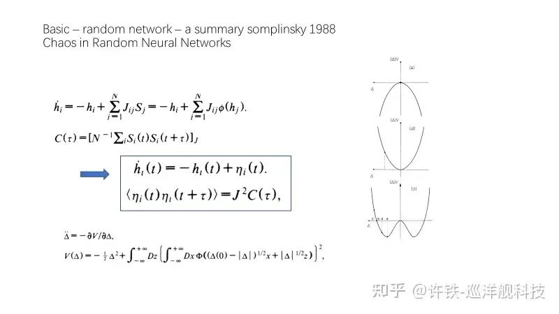
RNNs, or Recurrent Neural Networks, are an important theoretical tool in both machine learning and computational neuroscience.
In today’s world dominated by transformers, many may have forgotten about RNNs. However, RNNs remain a fundamental type of neural network and will surely play a role in the era of large models. First, let’s look at the structural differences between RNNs and convolutional networks (CNNs), which have established their prowess in processing static variables like images. The term “recurrent” highlights the core feature of RNNs, where the system’s output is retained in the network and combined with the system’s next input to determine the output at the next moment. This embodies the essence of dynamics, as recurrence corresponds to the feedback concept in dynamic systems, capable of depicting complex historical dependencies. From another perspective, this aligns with the famous Turing machine principle. The current state contains the history of the previous moment and serves as the basis for the next moment’s changes. This actually encompasses the core concept of programmable neural networks: when you have an unknown process, but you can measure the input and output, you assume that as this process goes through an RNN, it can learn the input-output patterns on its own, thus possessing predictive capabilities. In this respect, RNNs are Turing complete.

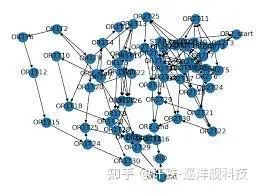
The core of RNNs lies in the network that describes the recurrence itself – W. W represents a map of connections between neurons, akin to a vast network of relationships. When an external response occurs, the neurons respond internally through this network, creating a complex symphony that resonates with external information and the network’s internal activities. This is the dynamics of RNNs, which allows the network to perform different tasks. This has significant implications for understanding biological phenomena and the essence of intelligence.
The W matrix itself can be viewed as a form of internal activity or a type of long-term memory. Its matrix characteristics determine the dynamics of RNNs. The analysis of this W is mathematically quite challenging because the matrix is too large, and under most conditions, it characterizes what we usually refer to as high-dimensional dynamic systems.
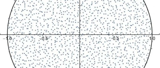
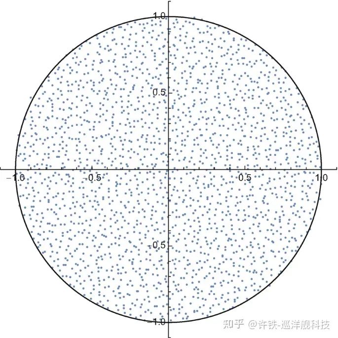
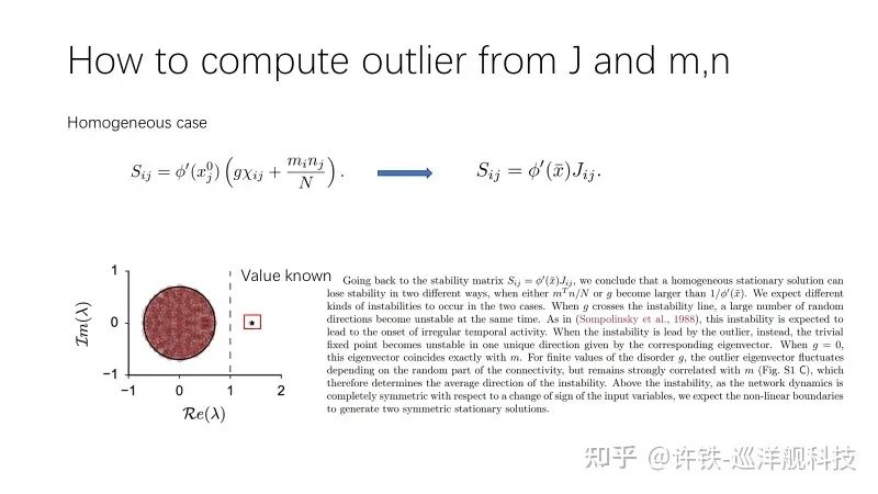
This high-dimensionality may sound abstract, but it essentially means that under any kind of input, the output we obtain is very difficult to predict; minor historical changes can lead to unpredictable subsequent variations – this is what we commonly refer to as chaos. The mathematical essence of this chaos is provided by random matrix theory, which states that the spectral distribution of random matrices is circular, and the radius of this circle determines the dynamics of the network (a smaller radius results in a steady state of zero activity, while exceeding a threshold leads to an approximately random chaotic state).
Due to its high intrinsic dimensionality, the network possesses a rich expressive capability, responding organically to different input histories to yield distinct internal neuronal activity trajectories. By utilizing the required output matrix, we can obtain the corresponding function we need. This property is often used to construct reservoir computing. We can view such a network as a universal network; however, it is regrettable that the predictive nature of such high-dimensional networks is not particularly adept.
Chaos possesses rich computational characteristics:
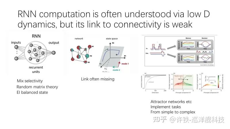
However, this inherently random network has been shown not to be the optimal solution post-learning. We find that RNNs that have been trained typically exhibit a reduction in dimensionality, while the tasks learned are also usually low-dimensional. What is the mathematical foundation behind this phenomenon?
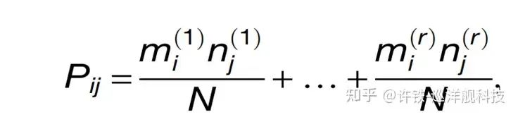
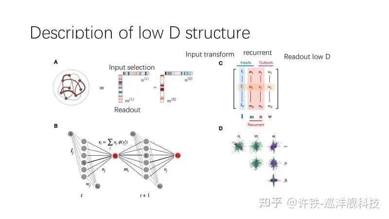
Experts from the Ostojic group at the École Normale Supérieure in Paris discovered that although high-dimensional matrices appear very high-dimensional, only a small portion of information is needed to control the dynamics of the entire network and achieve the corresponding task capabilities. This small portion of information is referred to as a low-rank matrix (P). For instance, a rank-one matrix is obtained by multiplying a left vector and a right vector. Although the matrix has many rows and columns, its actual dimensionality is only 1. If several such matrices are stacked, they form a low-rank matrix of rank n. We can also view the addition of this small portion of information as a form of disturbance, and the product form is a common characteristic of various network learning theories (first-order learning). This n typically determines the dimensionality of the subsequent dynamic system.
Why can the addition of this low-rank component control the entire dynamics? Because we say that high-dimensional matrices, despite their dimensionality, are random; each neuron exists under the unordered forces exerted by numerous surrounding neurons. Although these forces are numerous, when summed, they may leave little effect. In contrast, the information contained in low-rank matrices is deterministic and non-random, akin to islands in an ocean, standing out despite their scarcity. Each can exert an effective force on different neurons, thereby establishing the equilibrium position of the entire network.
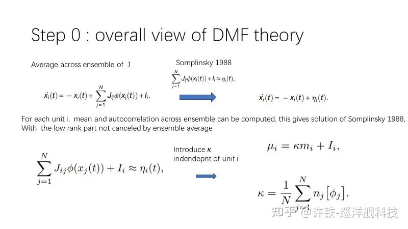
The entire mathematical analysis is provided by self-consistent mean-field theory. Simply put, it is the effect one has on those around them, which in turn affects oneself; this repeated interaction inevitably leads to an equivalent equilibrium position determined by the low-rank matrix associations between neurons. Therefore, the fate of the entire network is derived from the mean-field equations. The action of this equivalent field ensures that even in a non-chaotic state, the network does not trend towards a trivial solution where all neurons are inactive, but rather maintains a non-trivial steady state, or what we refer to as structural activity. In the chaotic vicinity, there exists a coexistence of chaotic inactivity and ordered activity, a characteristic not present in the dynamics caused by purely random matrices. Just a one-dimensional low-rank matrix can lead to this non-trivial fixed point, endowing the network with a series of complex nonlinear characteristics.
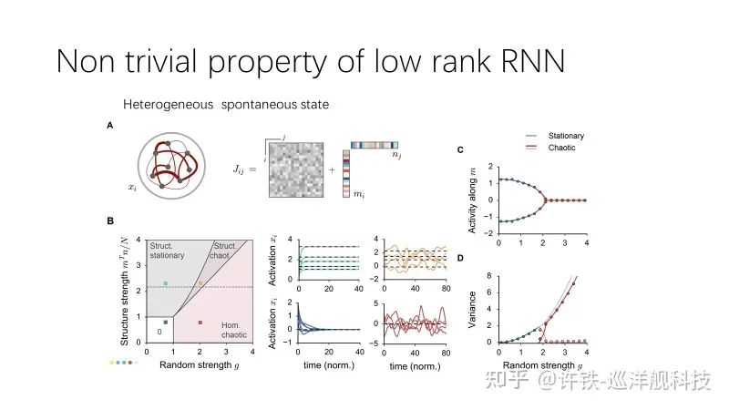
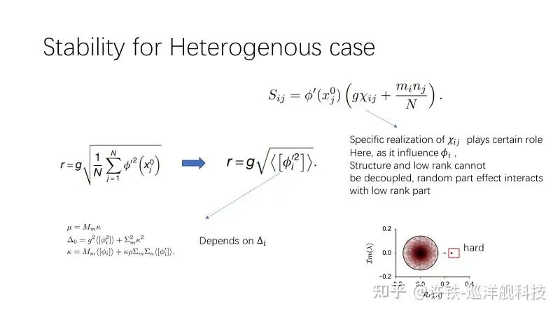
We say that the true computational characteristics of RNNs do not depend on the fixed point itself, but are given by the dynamic flows around the fixed point. These dynamic flows can usually be glimpsed through stability analysis theory. So, what is the mathematical principle here? The most important conclusion is that the random components of the network and the low-rank components jointly affect the entire network, leading to dynamics related to stability. This indicates that although the random components of the network are less important than the low-rank part, they cannot be overlooked. Their perturbative nature around the fixed point is evident, much like seawater battering the islands, where the islands represent the low-rank components and the seawater symbolizes the random components, which can even submerge the islands during high tides.
Next, we come to the most crucial part: how the input of the network affects the entire network. We say that the activity of the network under external input is the key factor influencing the network’s task capabilities. The previously discussed response of the network without external input can be seen as a ground state, while with external stimulation, the network enters an excited state. The relationship between this excited state and the ground state is essential to study. However, it is unfortunate that this analytical framework has not yet been mentioned in the field of large models.

We say that the most fundamental role of input is to transition the RNN from one dynamic region to another, making the input act like a switch, allowing the network to achieve two different states: on and off.
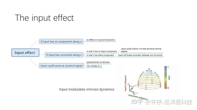
This state switching can also be understood from the perspective of symmetry breaking in physics, where external forces lead to a breaking of symmetry. Under this influence, the network can perform tasks similar to “go-nogo” tasks (for example, upon command, you must compare two different signals or count their quantities). Under a controlled variable input, the system transitions from one phase to another (go no-go stimulus), while another input that requires integration can yield different response functions across the two phases. Simultaneously, the network obtains the required output through a readout function (usually viewed as a vector multiplied by the network’s hidden state) (Here, there is another layer of control, where the direction of the readout vector and the left and right vectors of the low-rank matrix can determine whether to ignore or read out; if they are perpendicular, it indicates that the network’s activity is irrelevant to the readout; otherwise, it reads out, allowing the network to perform different tasks through different readouts). Thus, the network can achieve a series of nonlinear tasks.

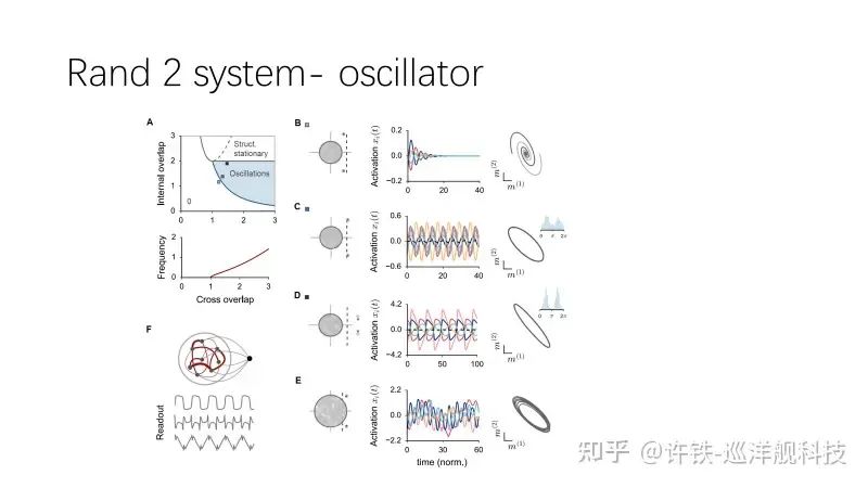
Previously, we only discussed one-dimensional systems (different stable points with varying stability under input influence). Through just a one-dimensional disturbance, the network can already accomplish many basic tasks. For two-dimensional systems, the structure of this dynamics can take on even more forms, such as limit cycles, which involve vibrations with different frequencies. In general, such dynamic systems can perform a wider variety of tasks.
Significance of Low-Rank Theory:
(1) Many complex biological systems can be viewed as high-dimensional dynamic systems controlled by complex W matrices, whether it is our nervous system or the massive molecular machinery of DNA. These systems change under external stimuli – and the external stimuli often originate from low-dimensional physical systems, such as mechanical motion in three-dimensional spacetime. In this process, the network itself undergoes a change – we usually refer to it as learning, typically exemplified by Hebbian learning in biology. The changes caused by this learning introduce an ordered low-dimensional component into the originally low-dimensional random network, which is the low-rank matrix. This low-rank matrix allows the properties or intelligence exhibited by organisms to possess highly ordered and structured characteristics. At the same time, I interpret this contraction of high-dimensional dynamics as a fate; in biology, it loses its omnipotence and gains a specific network. This loss of omnipotence inevitably leads to simpler and more ordered activities. We cannot avoid this differentiation, but we will still miss that imaginative high-dimensional era.
(2) The gap between randomness and order may not be that significant; what we need is how to introduce a slight disturbance to achieve different orders.
(3) Learning itself may not be as difficult or mysterious; by adding a small disturbance to the vast randomness, the network can exhibit various states, ultimately adapting to their respective environments.
References: Linking Connectivity, Dynamics, and Computations in Low-Rank Recurrent Neural Networks
Further Reading
When RNN Meets Reinforcement Learning – Establishing General Models for Space
The RNN Manual
Small and Beautiful Intelligence – Discussing Reservoir Computing