
Source: Deep Learning Enthusiasts

This article is about 3000 words long and is recommended to be read in 10 minutes.
This article introduces the basic components of CNN and classic network structures.
Author丨zzq@Zhihu
Link丨https://zhuanlan.zhihu.com/p/68411179
1. Introduction to Basic Components of CNN
In images, the connections between local pixels are relatively close, while the connections between distant pixels are relatively weak. Therefore, each neuron does not need to perceive the entire image globally; it only needs to perceive local information, which can then be combined at higher levels to obtain global information. The convolution operation is the realization of the local receptive field, and because convolution operations can share weights, it also reduces the number of parameters.
2. Pooling
Pooling reduces the input image size, decreases pixel information, and retains only important information, mainly to reduce computational load. It mainly includes max pooling and average pooling.
3. Activation Function
The activation function is used to introduce non-linearity. Common activation functions include sigmoid, tanh, and ReLU; the first two are often used in fully connected layers, while ReLU is common in convolutional layers.
4. Fully Connected Layer
The fully connected layer acts as a classifier in the entire convolutional neural network. The outputs from previous layers need to be flattened before entering the fully connected layer.
2. Classic Network Structures
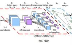
1. LeNet5
Consists of two convolutional layers, two pooling layers, and two fully connected layers. The convolution kernels are all 5×5, stride=1, and the pooling layer uses max pooling.

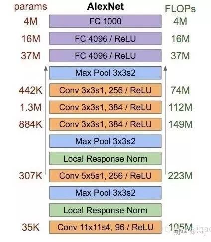
2. AlexNet
The model consists of eight layers (not counting the input layer), including five convolutional layers and three fully connected layers. The last layer uses softmax for classification output.
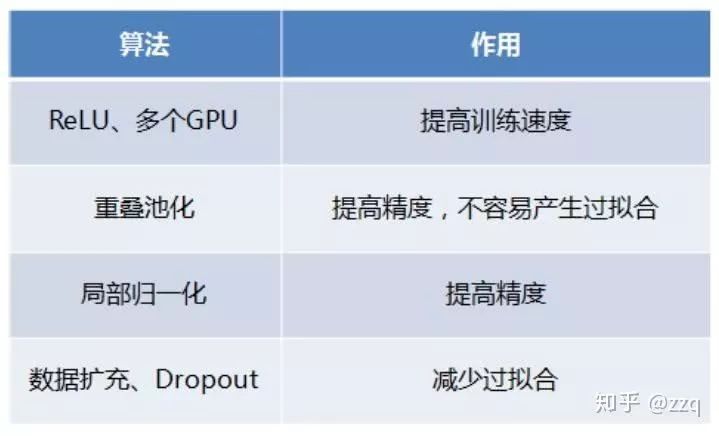
AlexNet uses ReLU as the activation function; it employs dropout and data augmentation to prevent overfitting; it implements dual GPUs; and it uses LRN.
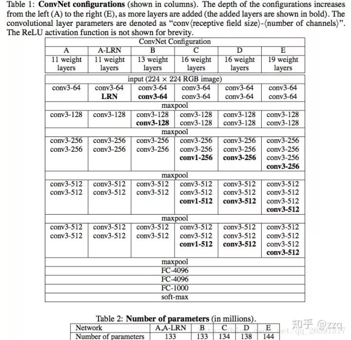
3. VGG
It uses a stack of 3×3 convolution kernels to simulate a larger receptive field and has a deeper network. VGG has five segments of convolution, each followed by a max pooling layer. The number of convolution kernels increases gradually.
Summary: LRN has little effect; deeper networks perform better; 1×1 convolutions are also effective but not as good as 3×3.
4. GoogLeNet (Inception v1)
From VGG, we learned that deeper networks perform better. However, as the model gets deeper, the number of parameters increases, leading to easier overfitting and requiring more training data. Additionally, complex networks imply more computational load and larger model storage needs, which require more resources and reduce speed. GoogLeNet is designed to reduce parameters.
GoogLeNet increases network complexity by widening the network, allowing the network to choose how to select convolution kernels itself. This design reduces parameters while enhancing the network’s adaptability to multiple scales. Using 1×1 convolutions allows for increased network complexity without adding parameters.

Inception-v2
On the basis of v1, batch normalization technology is added. In TensorFlow, using BN before the activation function yields better results; the 5×5 convolution is replaced with two consecutive 3×3 convolutions to make the network deeper with fewer parameters.
Inception-v3
The core idea is to decompose convolution kernels into smaller convolutions, for example, decomposing 7×7 into 1×7 and 7×1 convolutions to reduce network parameters and increase depth.
Inception-v4 Structure
Introduced ResNet to accelerate training and improve performance. However, when the number of filters is too large (>1000), training becomes very unstable; an activation scaling factor can be added to alleviate this.
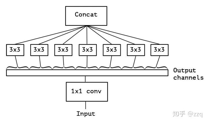
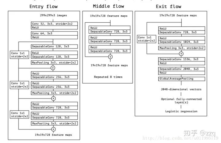
5. Xception
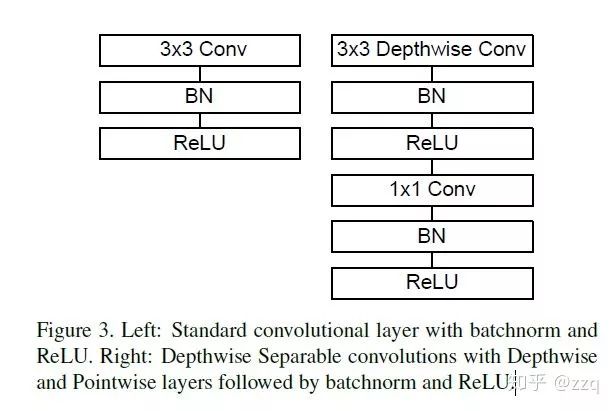
Based on Inception-v3, the basic idea is depthwise separable convolution but with differences. The model parameters are slightly reduced, but the accuracy is higher. Xception first performs a 1×1 convolution followed by a 3×3 convolution, i.e., merging channels first, then performing spatial convolution. Depthwise is the opposite, first performing spatial 3×3 convolution, then 1×1 convolution on channels. The core idea is to follow an assumption: during convolution, the convolution of channels should be separated from the spatial convolution. MobileNet-v1 uses the depthwise order and adds BN and ReLU. The parameter count of Xception is not much different from Inception-v3; it increases network width to enhance accuracy, while MobileNet-v1 aims to reduce parameters and improve efficiency.
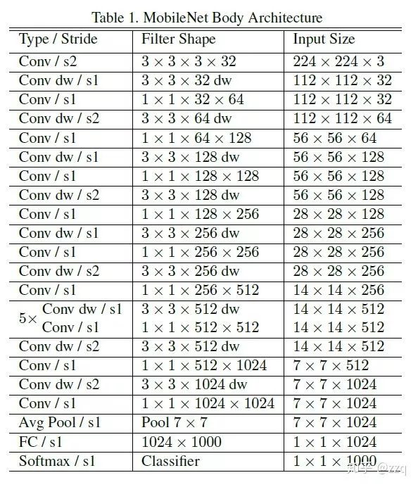
6. MobileNet Series
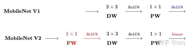
V1
Uses depthwise separable convolutions; abandons pooling layers and uses stride=2 convolutions. The number of channels in standard convolution kernels equals the number of input feature map channels; while the depthwise convolution kernel channel count is 1; there are two parameters that can be controlled, a controls input-output channel count; p controls image (feature map) resolution.
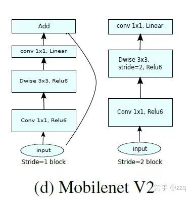
V2
Compared to v1, there are three differences: 1. Introduced residual structure; 2. Before dw, a 1×1 convolution is performed to increase the feature map channel count, which is different from the general residual block; 3. After pointwise, ReLU is abandoned in favor of a linear activation function to prevent ReLU from damaging features. This is because the features extracted by the dw layer are limited by the input channel count; if the traditional residual block is used, the features that dw can extract are even less. Therefore, initially not compressing but rather expanding is the approach. However, when using expansion-convolution-compression, a problem arises after compression: ReLU can damage features, and since features are already compressed, passing through ReLU will lose some features, so linear should be used.
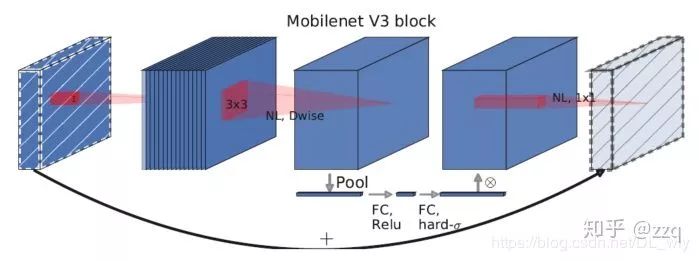
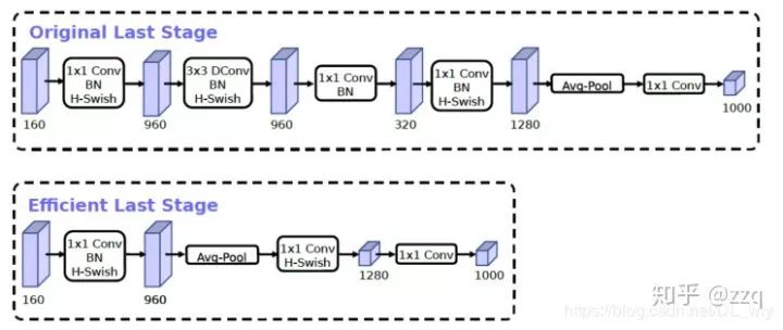
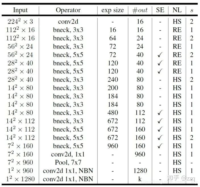
V3
Complementary search technology combination: executed by resource-constrained NAS module set search, NetAdapt performs local searches; network structure improvements: move the last average pooling layer forward and remove the last convolution layer, introduce h-swish activation function, modified the initial filter group.
V3 integrates the depthwise separable convolutions of v1, the linear bottleneck residual structure of v2, and the lightweight attention model of SE structure.
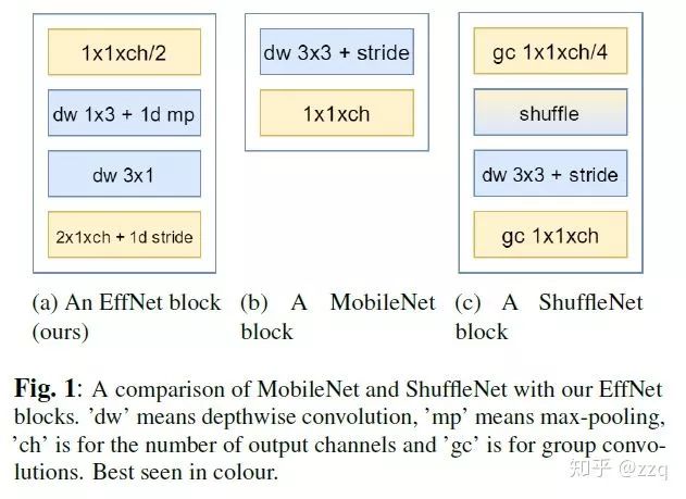
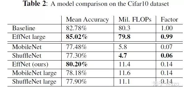
7. EffNet
EffNet is an improvement on MobileNet-v1, with the main idea: decompose the dw layer of MobileNet-1 into two 3×1 and 1×3 dw layers, so that pooling is adopted after the first layer, thereby reducing the computational load of the second layer. EffNet is smaller and progresses faster than MobileNet-v1 and ShuffleNet-v1 models.
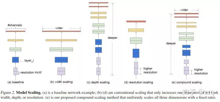
8. EfficientNet
Research on expanding network design in depth, width, and resolution, and the interrelationships between them. Higher efficiency and accuracy can be achieved.
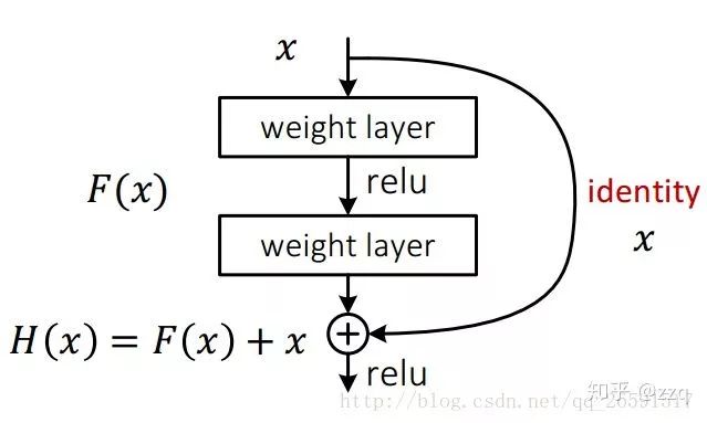
9. ResNet
VGG proved that deeper networks are an effective means of improving accuracy, but deeper networks can easily lead to gradient vanishing, making it difficult for the network to converge. Tests showed that more than 20 layers resulted in increasingly poor convergence with increasing layers. ResNet can effectively address the gradient vanishing problem (actually alleviating it, not truly solving it) by adding shortcut connections.
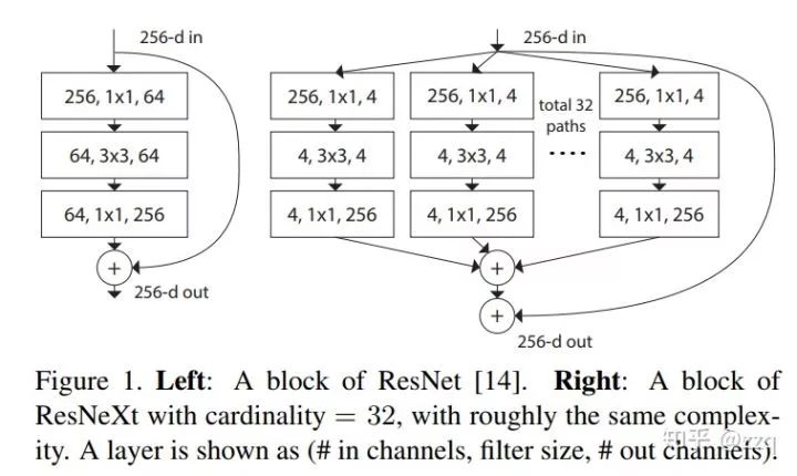
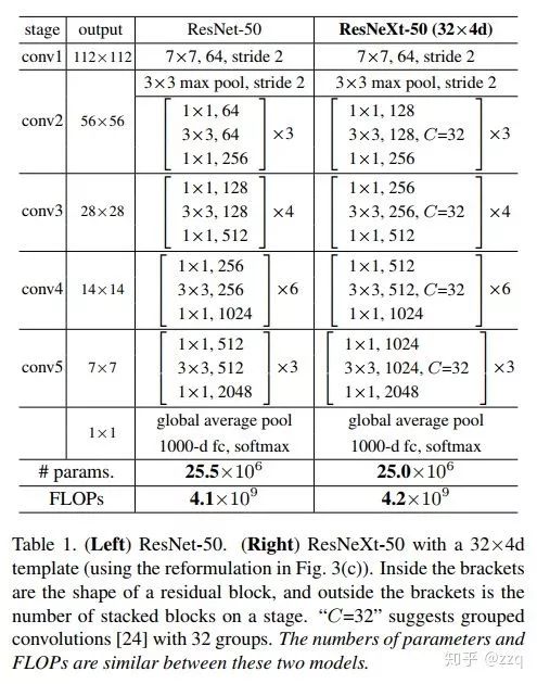
10. ResNeXt
Based on ResNet and Inception’s split+transform+concatenate combination. However, it performs better than ResNet, Inception, and Inception-ResNet. Group convolution can be used. Generally, there are three ways to increase network expressive power: 1. Increase network depth, such as from AlexNet to ResNet, but experimental results show that the improvement brought by network depth becomes smaller; 2. Increase the width of network modules, but increasing width inevitably leads to exponential parameter scale increases, which is not mainstream CNN design; 3. Improve CNN network structure design, such as Inception series and ResNeXt. Experiments found that increasing cardinality, i.e., the number of identical branches in a block, can better enhance model expressive power.
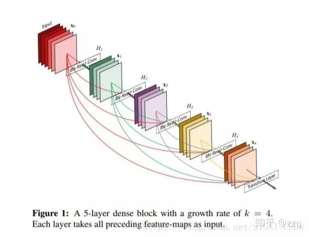
11. DenseNet
DenseNet significantly reduces the number of parameters through feature reuse and alleviates the gradient vanishing problem to some extent.
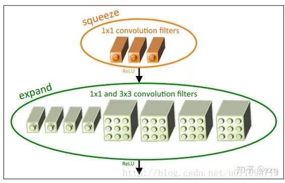
12. SqueezeNet
Proposed the fire-module: squeeze layer + expand layer. The squeeze layer is a 1×1 convolution, and the expand layer uses both 1×1 and 3×3 convolutions, followed by concatenation. SqueezeNet has 1/50 the parameters of AlexNet and after compression is 1/510, but the accuracy is comparable to AlexNet.
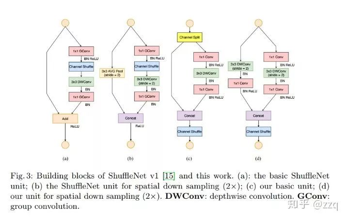
13. ShuffleNet Series
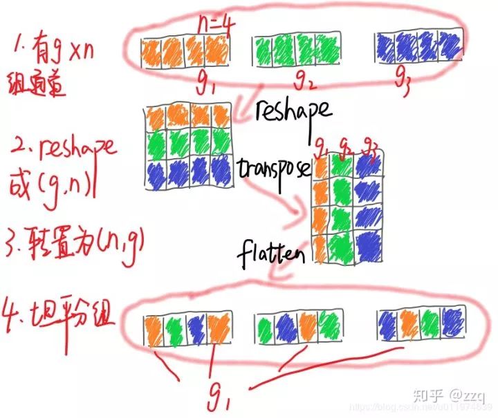
V1
Reduces computational load through grouped convolutions and 1×1 pointwise group convolution kernels, enriching the information of each channel through channel reorganization. Xception and ResNeXt are inefficient in small network models due to the high resource consumption of numerous 1×1 convolutions; therefore, pointwise group convolution is proposed to reduce computational complexity. However, using pointwise group convolution has side effects, so channel shuffle is proposed to aid information flow. Although dw can reduce computation and parameter count, its efficiency in low-power devices is worse than dense operations, thus ShuffleNet aims to use depthwise convolutions at bottlenecks to minimize overhead.
V2
Design criteria for making neural networks more efficient:
-
Keeping the number of input channels equal to the number of output channels can minimize memory access costs; -
Using too many groups in grouped convolutions increases memory access costs; -
Overly complex network structures (too many branches and basic units) reduce the network’s parallelism; -
Element-wise operations are also not negligible.
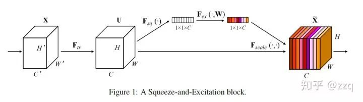
14. SENet
15. SKNet

Editor: Huang Jiyuan
