
Continuing from the previous article Deep Learning (1) – Overview, Distributed Representation, and Ideas
9. Common Models or Methods in Deep Learning
9.1 AutoEncoder
The specific process is briefly described as follows:
1) Given unlabeled data, learn features using unsupervised learning:
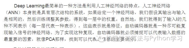
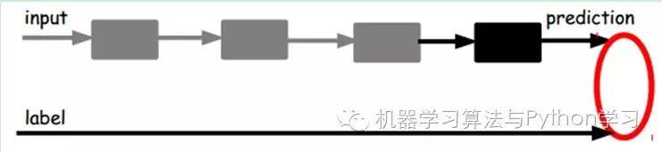
In our previous neural network, as shown in the first diagram, the samples we input are labeled, i.e., (input, target), so we change the parameters of the previous layers based on the difference between the current output and the target (label) until convergence. However, now we only have unlabeled data, which is shown in the right diagram. So how do we obtain this error?
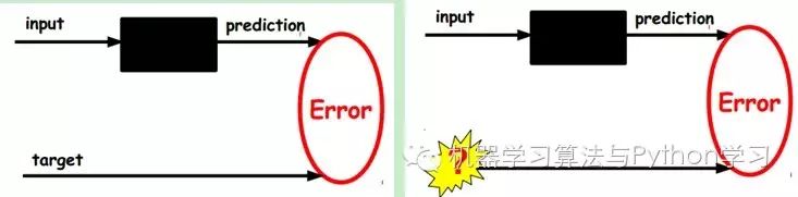
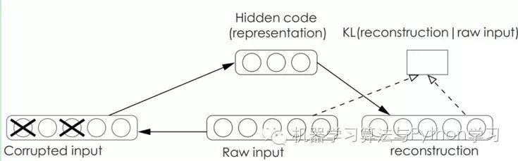
As shown in the diagram above, we input the input into an encoder, which will yield a code; this code represents the input. How do we know this code represents the input? We add a decoder, which will output a message. If this output is very similar to the original input signal (ideally, it should be identical), then we have reason to believe that this code is reliable. Thus, we adjust the parameters of the encoder and decoder to minimize the reconstruction error, at which point we obtain the first representation of the input signal, which is the code. Since it is unlabeled data, the source of error comes directly from comparing the reconstruction with the original input.
2) Generate features through the encoder and then train the next layer. Train layer by layer:
From the above, we have obtained the code for the first layer. Our minimized reconstruction error allows us to believe that this code is a good representation of the original input signal, or to put it a bit loosely, it is identical to the original signal (different representations reflect the same thing). The training method for the second layer is no different from that of the first layer; we take the code output from the first layer as the input signal for the second layer and minimize the reconstruction error to obtain the parameters for the second layer and the code for the second layer’s input, which is the second representation of the original input information. The same method applies to other layers (train this layer while fixing the parameters of the previous layers, and their decoders are no longer needed).
3) Supervised fine-tuning:
After the above methods, we can obtain many layers. As for how many layers (or how deep), there is currently no scientific evaluation method, and you need to experiment yourself. Each layer will obtain different representations of the original input. Of course, we believe that the more abstract, the better, just like the human visual system.
At this point, the AutoEncoder still cannot be used to classify data, as it has not yet learned how to connect an input with a class. It has only learned how to reconstruct or reproduce its input. In other words, it has only learned to obtain a feature that can well represent the input signal. To achieve classification, we can add a classifier (e.g., logistic regression, SVM, etc.) at the top coding layer of the AutoEncoder, and then train it using standard supervised training methods for multilayer neural networks (gradient descent).
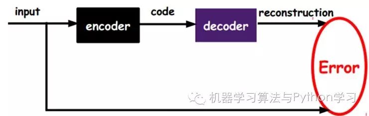
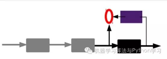
That is to say, at this point, we need to input the feature code from the final layer into the final classifier and fine-tune it through labeled samples using supervised learning, which can be done in two ways: one is to adjust only the classifier (the black part):
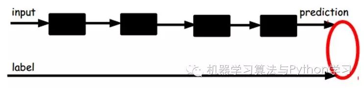
The other way: fine-tune the entire system through labeled samples (if there is enough data, this is the best. End-to-end learning).
Once the supervised training is completed, this network can be used for classification. The top layer of the neural network can serve as a linear classifier, and we can replace it with a better-performing classifier.
Research has shown that if we add these automatically learned features to the original features, it can significantly improve accuracy, even outperforming the best current classification algorithms in classification problems!
The AutoEncoder has some variants; here are brief introductions to two:
Sparse AutoEncoder:
Of course, we can also add some constraints to obtain new Deep Learning methods. For example, if we add an L1 Regularity constraint (L1 mainly constrains that most nodes in each layer must be 0, with only a few non-zero, which is the source of the name Sparse) to the AutoEncoder, we can obtain the Sparse AutoEncoder method.
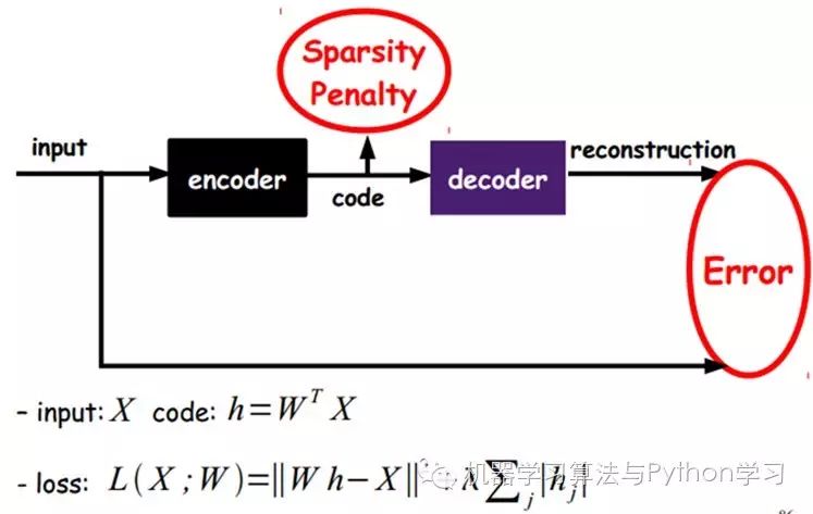
As shown in the diagram, it actually restricts each expression code obtained to be as sparse as possible. Sparse representations are often more effective than other representations (the human brain seems to work this way, where a certain input only stimulates certain neurons, while most other neurons are inhibited).
Denoising AutoEncoders:
Denoising AutoEncoders (DA) are based on AutoEncoders but add noise to the training data, so the AutoEncoder must learn to remove this noise to obtain the true input that has not been contaminated by noise. This forces the encoder to learn a more robust representation of the input signal, which is also why its generalization ability is stronger than that of ordinary encoders. DA can be trained using gradient descent algorithms.
9.3 Restricted Boltzmann Machine (RBM)
Assume there is a bipartite graph, where there are no links between nodes in each layer. One layer is the visible layer, i.e., the input data layer (v), and the other layer is the hidden layer (h). If we assume that all nodes are random binary variable nodes (can only take values of 0 or 1), and that the joint probability distribution p(v,h) satisfies the Boltzmann distribution, we call this model the Restricted Boltzmann Machine (RBM).
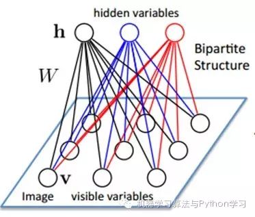
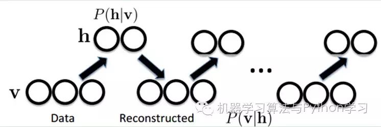
Let’s see why it is a Deep Learning method. First, because this model is a bipartite graph, the hidden nodes are conditionally independent of each other given v (because there are no connections between nodes), i.e., p(h|v)=p(h1|v)…p(hn|v). Similarly, given the hidden layer h, all visible nodes are conditionally independent. Also, since all v and h satisfy the Boltzmann distribution, when inputting v, we can obtain the hidden layer h through p(h|v), and after obtaining the hidden layer h, we can get the visible layer through p(v|h). By adjusting the parameters, we aim to make the visible layer v1 obtained from the hidden layer identical to the original visible layer v. Thus, the hidden layer can serve as a feature of the visible layer input data, making it a Deep Learning method.
How to train? Specifically, how to determine the weights between the visible layer nodes and the hidden nodes? We need to perform some mathematical analysis. This is the model.
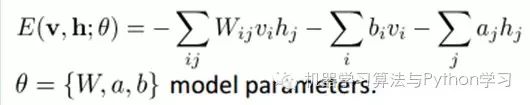
The energy of the joint configuration can be expressed as:
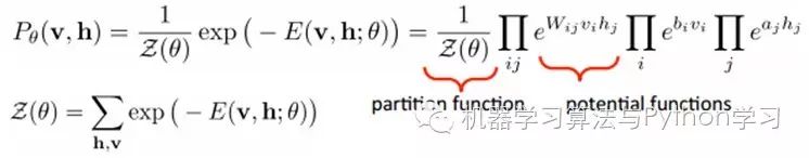
The joint probability distribution for a certain configuration can be determined by the Boltzmann distribution (and the energy of this configuration):
Since the hidden nodes are conditionally independent (because there are no connections between nodes), i.e.,
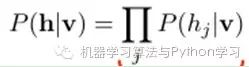
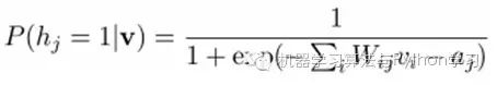
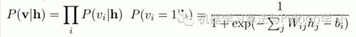
Then we can easily (factorize the above expression) obtain the probability of the j-th hidden node being 1 or 0 given the visible layer v:
Similarly, given the hidden layer h, the probability of the i-th visible node being 1 or 0 can also be easily obtained:
Given a sample set D={v(1), v(2),…, v(N)} that satisfies independent and identically distributed, we need to learn the parameters θ={W,a,b}.
We maximize the following log-likelihood function (maximum likelihood estimation: for a certain probability model, we need to choose a parameter that maximizes the probability of our current observed samples):
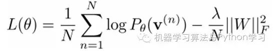
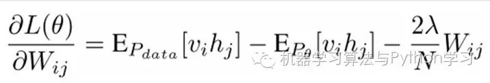
That is, by taking the derivative of the maximum log-likelihood function, we can obtain the parameters W when L is maximized.
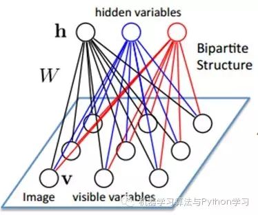
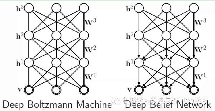
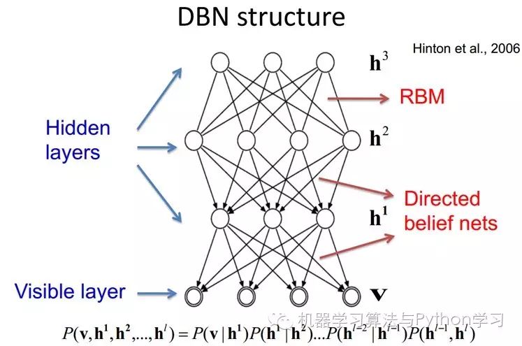
If we increase the number of hidden layers, we can obtain a Deep Boltzmann Machine (DBM); if we use Bayesian belief networks (i.e., directed graphical models, while still ensuring no connections between nodes in the layer) near the visible layer and use Restricted Boltzmann Machines in the parts farthest from the visible layer, we can obtain Deep Belief Networks (DBN).
9.4 Deep Belief Networks
DBNs are a probabilistic generative model, in contrast to traditional discriminative models of neural networks. Generative models establish a joint distribution between observed data and labels, evaluating both P(Observation|Label) and P(Label|Observation), while discriminative models only evaluate the latter, i.e., P(Label|Observation). When applying traditional BP algorithms in deep neural networks, DBNs encounter the following issues:
(1) Requires a labeled sample set for training;
(2) Slow learning process;
(3) Improper parameter selection can lead to convergence to local optimal solutions.
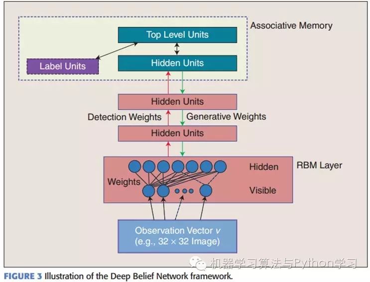
DBNs consist of multiple layers of Restricted Boltzmann Machines (RBMs), a typical neural network type as shown in Figure 3. These networks are “restricted” to one visible layer and one hidden layer, with connections between layers but no connections between units within layers. The hidden layer units are trained to capture the high-order correlations of the data manifested in the visible layer.
First, without considering the top two layers that form an associative memory, the connections of a DBN are guided by generative weights from top to bottom. RBMs serve as building blocks; compared to traditional and deep-layered sigmoid belief networks, they facilitate the learning of connection weights.
Initially, a greedy layer-wise unsupervised pre-training method is used to obtain the generative model weights, which has been proven effective by Hinton and termed Contrastive Divergence.
In this training phase, a vector v is generated at the visible layer, which transmits values to the hidden layer. Conversely, the input of the visible layer will be randomly selected to attempt to reconstruct the original input signal. Finally, these new visible neuron activation units will forward pass to reconstruct the hidden layer activation units, obtaining h (in the training process, the visible vector values are first mapped to the hidden units; then the visible units are reconstructed by the hidden layer units; these new visible units are mapped back to the hidden units, thus obtaining new hidden units. This repetitive process is called Gibbs sampling). These backward and forward steps are what we know as Gibbs sampling, and the correlation difference between hidden layer activation units and visible layer inputs serves as the main basis for weight updates.
Training time is significantly reduced because only a single step is needed to approach maximum likelihood learning. Adding each layer to the network improves the log probability of the training data, which we can understand as getting closer to the true expression of energy. This meaningful extension and the use of unlabeled data are decisive factors for any deep learning application.
In the top two layers, weights are connected together, so the outputs from lower layers provide a reference clue or association to the top layer, which will connect it to its memory content. What we care most about is the final discriminative performance, such as in classification tasks.
After pre-training, the DBN can use labeled data to adjust its discriminative performance using the BP algorithm. Here, a label set will be attached to the top layer (promoting associative memory), obtaining a network classification boundary through a bottom-up learned recognition weight. This performance will be better than a network trained solely by the BP algorithm. This can be intuitively explained: the BP algorithm of DBNs only requires a local search of the weight parameter space, which is faster and requires less convergence time compared to feedforward neural networks.
The flexibility of DBNs makes them easier to extend. One extension is Convolutional DBNs (CDBNs). DBNs do not consider the 2D structural information of images because the input is simply vectorized from a 2D image matrix. CDBNs address this issue by utilizing the spatial relationships of neighboring pixels, achieving transformation invariance through a model called Convolutional RBMs, and can easily transform to high-dimensional images. DBNs do not explicitly handle the learning of temporal relationships of observed variables, although there has been research in this area, such as stacking temporal RBMs, leading to a sequence learning method dubbed temporal convolution machines. This application of sequence learning presents an exciting future research direction for speech signal processing.
Currently, research related to DBNs includes stacked AutoEncoders, which replace the RBMs in traditional DBNs with stacked AutoEncoders. This allows for the training of deep multilayer neural network architectures using the same rules, but it lacks the strict parameterization requirements of layers. Unlike DBNs, AutoEncoders use discriminative models, making it challenging for this structure to sample the input space, which makes it harder for the network to capture its internal representation. However, Denoising AutoEncoders can effectively avoid this problem and outperform traditional DBNs. They achieve this by adding random noise during the training process and stacking to enhance generalization performance. The training process of a single Denoising AutoEncoder is similar to that of training RBMs for generative models.
 Thank you for your attention and support
Feel free to reprint