Comprehensive Overview of RNN (Recurrent Neural Networks)

Introduction to Recurrent Neural Networks

Why RNN After BP Algorithm and CNN?

Upon reflection on the BP algorithm and CNN (Convolutional Neural Networks), we find that their outputs only consider the influence of the previous input without taking into account the influence of inputs at other times. For instance, recognizing single objects like cats, dogs, or handwritten digits yields good results. However, for tasks related to temporal sequences, such as predicting the next moment in a video or understanding the context of a document, these algorithms perform inadequately. Hence, RNNs emerged.

What is RNN?

A Recurrent Neural Network (RNN) is a type of neural network that takes sequence data as input and recursively processes it in the direction of the sequence evolution, where all nodes (recurrent units) are connected in a chain-like fashion.

RNN is a special type of neural network structure that is based on the idea that human cognition is based on past experiences and memories. Unlike DNNs and CNNs, RNNs not only consider the previous input but also endow the network with a memory function for prior content.

The reason RNN is called a recurrent neural network is that the current output of a sequence is also related to previous outputs. Specifically, the network remembers previous information and applies it to the current output calculation, meaning that nodes between hidden layers are no longer unconnected but are connected, and the input to the hidden layer includes not only the output from the input layer but also the output from the previous hidden layer.

Application Areas

RNNs have numerous application areas; it can be said that as long as there is a consideration of the order of time, RNNs can be used to solve the problem. Here are a few common application areas:

① Natural Language Processing (NLP): including video processing, text generation, language models, image processing
② Machine translation, machine-generated novels
③ Speech recognition
④ Image caption generation
⑤ Text similarity computation
⑥ Music recommendation, product recommendations on platforms like NetEase Kaola, YouTube video recommendations, and other new application areas.

Development History

Representative RNNs

• Basic RNN: The fundamental structure of recurrent networks
• LSTM: A breakthrough long short-term memory network
• GRU: A new type of cell module
• NTM: Exploring larger memory models

Network Popularity

Basic RNN

First, let’s look at a simple recurrent neural network shown below, which consists of an input layer, a hidden layer, and an output layer:

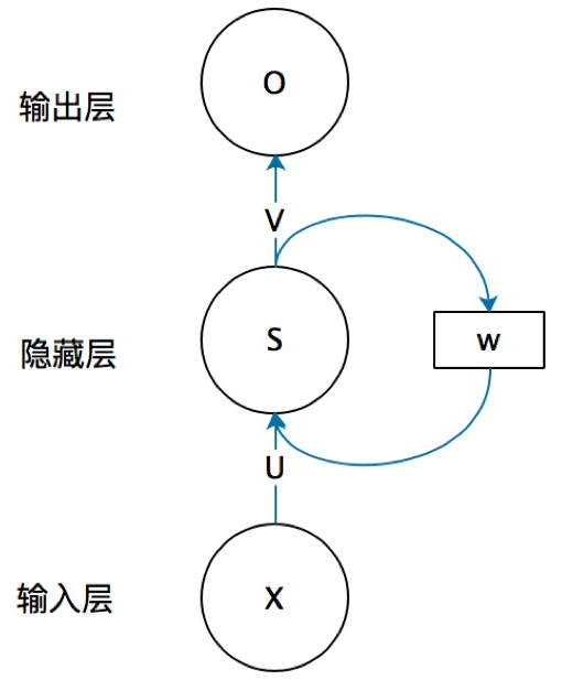
If we remove the arrowed circle with W, it becomes the most basic fully connected neural network.

• x is a vector representing the input layer values (the circles representing neuron nodes are not shown here);
• s is a vector representing the hidden layer output values (the hidden layer shows one node, but you can imagine that this layer actually consists of multiple nodes, with the number of nodes equal to the dimension of vector s);
• U is the weight matrix from the input layer to the hidden layer;
• o is also a vector representing the output layer values;
• V is the weight matrix from the hidden layer to the output layer.

Now, let’s see what W is. The value s of the hidden layer in the recurrent neural network not only depends on the current input x but also on the previous value s of the hidden layer. The weight matrix W serves as the weight for the previous value of the hidden layer as the input for the current instance. This is how the temporal memory function is implemented.

We provide a specific diagram corresponding to this abstract diagram:

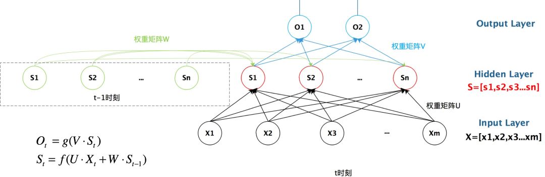
From the above diagram, we can clearly see how the previous hidden layer influences the current hidden layer.

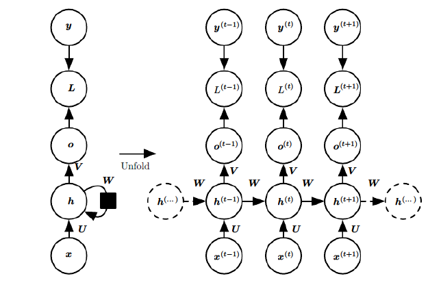
If we expand the above diagram, the recurrent neural network can also be represented as follows:

This is a standard RNN structure diagram, where each arrow represents a transformation, meaning that the arrows connect with weights. The left side shows a folded structure, while the right side shows an unfolded structure, where the arrows next to it represent how the “recurrent” nature is manifested in the hidden layer. In the unfolded structure, we can observe that in the standard RNN structure, the neurons in the hidden layer are also connected with weights. As the sequence progresses, previous hidden layers will influence subsequent hidden layers. The diagram represents the output, the determined values provided by the samples, and the loss function; we can see that the “loss” accumulates as the sequence progresses.

In addition to the above characteristics, the standard RNN also has the following features:

1. Weight sharing, where all Ws in the diagram are the same, and U and V are the same as well.
2. Each input value is only connected to its own path and does not connect to other neurons.
3. The hidden state can be understood as: h = f(current input + past memory summary)

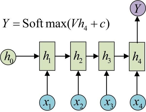
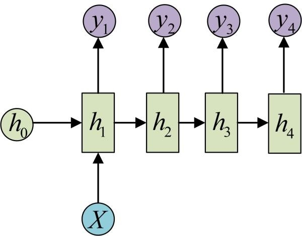
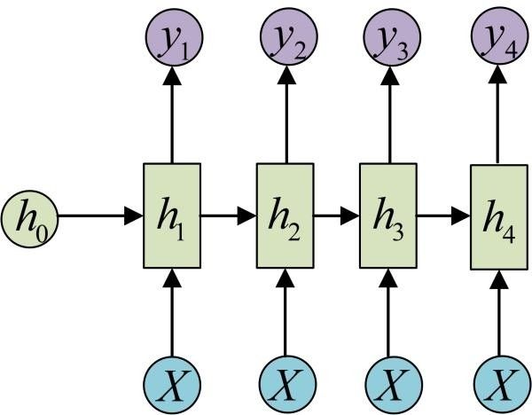
The above is the standard structure of RNN N VS N (N inputs correspond to N outputs), meaning that the input and output sequences must be of equal length.

Due to this limitation, the classic RNN has a relatively small applicable range, but there are still some problems suitable for modeling with the classic RNN structure, such as:

• Calculating the classification label for each frame in a video. Since each frame needs to be computed, the input and output sequences are of equal length.
• Inputting characters and outputting the probability of the next character. This is the famous Char RNN (for detailed introduction, please refer to: The Unreasonable Effectiveness of Recurrent Neural Networks; Char RNN can be used to generate articles, poetry, and even code, which is very interesting).

RNN Variants

N VS 1

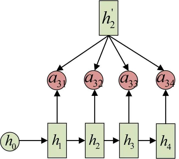
The standard structure of RNN N VS N cannot solve all problems in practice. Sometimes, we need to handle a situation where the input is a sequence and the output is a single value rather than a sequence. For example, if we input a string of text, the output is a classification category, then the output does not need to be a sequence, only a single output is needed. How should we model this? In fact, we only need to perform the output transformation at the last t.

This structure is usually used to address sequence classification problems. For instance, inputting a segment of text to determine its category, inputting a sentence to assess its sentiment, and inputting a video segment to determine its category, etc.

1 VS N

How to handle the case where the input is not a sequence but the output is a sequence? We can compute the input only at the beginning of the sequence:

Another structure uses the input information as input at each stage (the input is a sequence but does not change with the sequence):

The following diagram omits some circles of X, which is an equivalent representation:

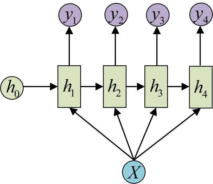
This 1 VS N structure can solve problems such as:

• Generating text from images (image captioning), where the input is the features of the image and the output sequence is a sentence;
• Generating speech or music from categories.

N VS M

Next, we introduce one of the most important variants of RNN: N vs M. This structure is also known as the Encoder-Decoder model, or Seq2Seq model.

The original N vs N RNN requires sequences to be of equal length; however, most of the problems we encounter involve sequences of unequal lengths, such as in machine translation, where the source and target language sentences often do not have the same length.

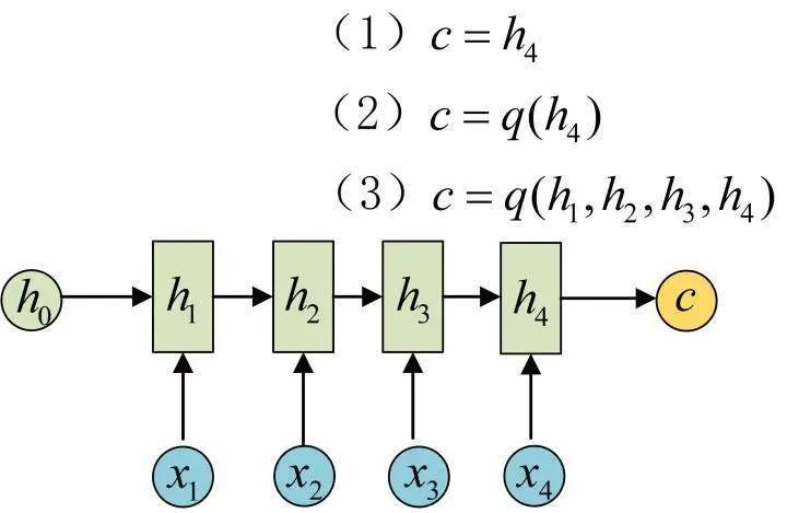
To address this, the Encoder-Decoder structure first encodes the input data into a context vector c:

This can be achieved in various ways, with the simplest method being to assign the last hidden state of the Encoder to c. It can also be transformed from the last hidden state or from all hidden states.

After obtaining c, another RNN network is used to decode it. This part of the RNN network is referred to as the Decoder. The specific approach is to input c as the initial state into the Decoder:

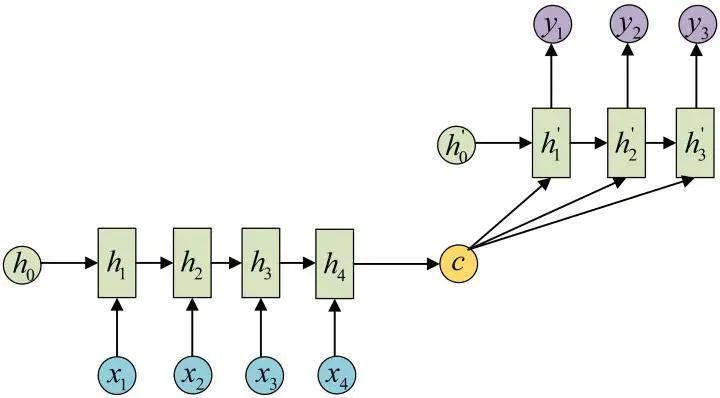
Another approach is to use c as the input for each step:

Because this Encoder-Decoder structure does not restrict the lengths of input and output sequences, its application range is very broad. For example:

• Machine translation. The Encoder-Decoder structure was first proposed in the field of machine translation;
• Text summarization. Input is a sequence of text, and output is a summary sequence of this text;
• Reading comprehension. The input article and question are encoded separately, and then decoded to obtain the answer to the question;
• Speech recognition. The input is a sequence of speech signals, and the output is a sequence of text.

Attention Mechanism

In the Encoder-Decoder structure, the Encoder encodes all input sequences into a unified semantic feature c for decoding, **thus, c must contain all the information from the original sequence, and its length becomes a bottleneck limiting the model’s performance.** For instance, in machine translation, when the sentence to be translated is long, a single c may not be able to hold enough information, leading to a drop in translation accuracy.

The Attention mechanism addresses this issue by inputting different c values at each time step. The following diagram shows the Decoder with the Attention mechanism:

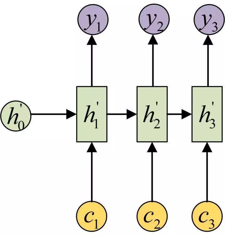
Each c will automatically select the most suitable contextual information for the current output. Specifically, we use α to measure the relevance between the j stage in the Encoder and the i stage in the Decoder, and ultimately, the input context information at the i stage in the Decoder comes from the weighted sum of all h related to j.

For example, in machine translation (translating Chinese to English):

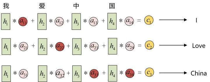
The input sequence is “I love China”, so the h in the Encoder can be seen as representing the information of “I”, “love”, “China”. When translating into English, the first context should be most relevant to the word “I”, thus the corresponding α is relatively large, while the h corresponding to “love” should be larger. Finally, the h corresponding to “China” should also be larger.

At this point, regarding the Attention model, we are left with one last question: how is α calculated?

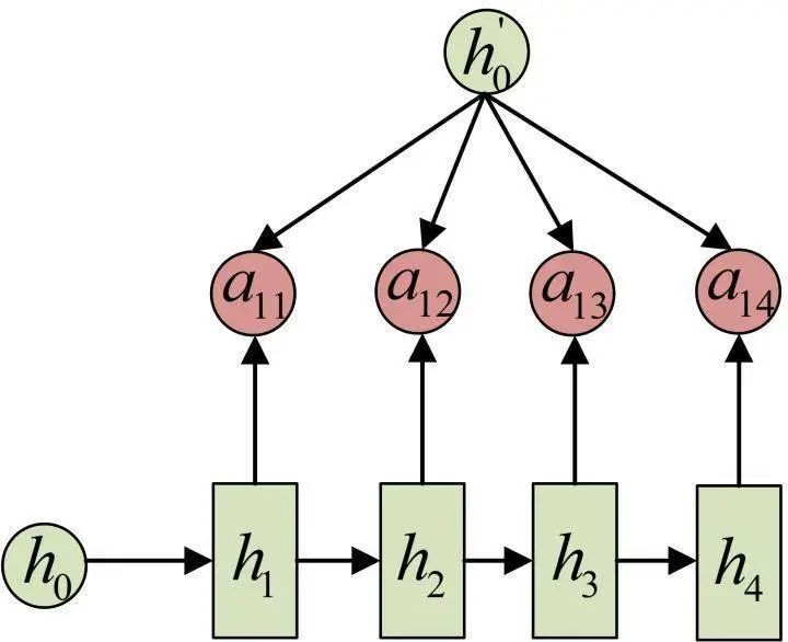
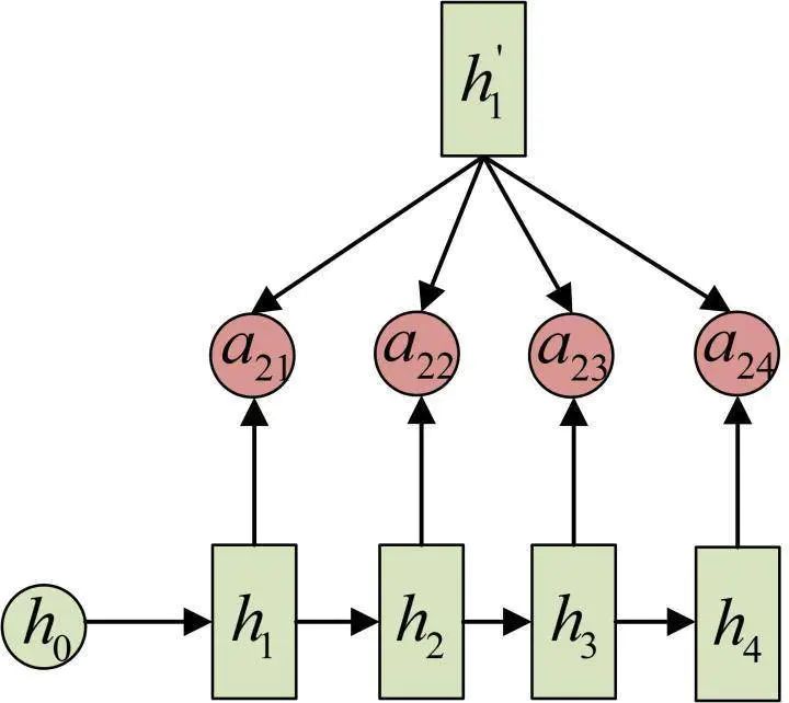
In fact, α is also learned from the model, and it is related to the hidden state at the i stage of the Decoder and the hidden state at the j stage of the Encoder.

Taking the above example of machine translation, the calculation of α (the arrows indicate transformations on h' and h):

The calculation of h:

The calculation of c:

This is the complete calculation process of the Encoder-Decoder model with Attention.

You may have noticed that there is no content on LSTM; this is because LSTM looks completely the same as RNN from the outside, so all the above structures are applicable to LSTM.

Forward Output Process of Standard RNN

The above introduced many variants of RNN, but their mathematical derivation processes are essentially similar. Here, we introduce the forward propagation process of the standard structure RNN.

Next, let’s introduce the meaning of each symbol: x is the input, h is the hidden layer unit, o is the output, L is the loss function, and y is the label of the training set. The elements with a superscript t represent the state at time t. It is important to note that the performance of the hidden unit h at time t is not only determined by the input at that moment but also affected by the previous moments. W is the weight, and weights of the same type are the same.

With the above understanding, the forward propagation algorithm is quite simple. For time t:

where ϕ is the activation function, generally, the tanh function is chosen, and b is the bias.

The output at time t is even simpler:

The final model’s predicted output is:

where σ is the activation function, and since RNN is generally used for classification, the softmax function is usually used here.

Equation (1) is the computation formula for the hidden layer, which is the recurrent layer. Equation (2) is the computation formula for the output layer, which is a fully connected layer.

From the above equations, we can see that the difference between the recurrent layer and the fully connected layer is that the recurrent layer has an additional weight matrix.

If we repeatedly substitute Equation (1) into Equation (2), first removing the bias, we will obtain:

From the above, it can be seen that the output value of the recurrent neural network, o, is influenced by the previous input values x, h, etc., which is why the recurrent neural network can look back at any number of input values.

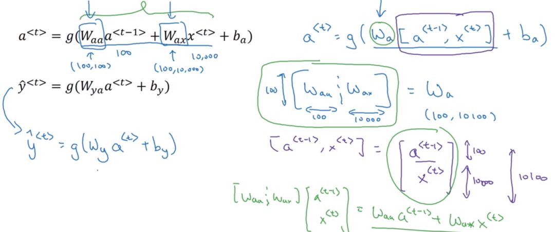
Sometimes Equation (1) is written in the following form:

This is because in Equation (3), h equals the vector, for example, if the shape of h is (10, 1), the shape of W is (10, 10), the shape of o is (20, 1), then the shape of W is (10, 20), and the final shape is (10, 1).

Looking at the shape of o as (10, 30), while the shape of h is (30, 1), then (10, 30) * (30, 1) = (10, 1), thus Equation (1) and Equation (3) are equivalent.

Here is a hand-derivation diagram by Andrew Ng:

Training Method for RNN – BPTT

BPTT (Back-Propagation Through Time) is a commonly used training method for RNNs. Essentially, it is still the BP algorithm, but since RNNs handle time series data, it needs to propagate backward through time, hence the name. The central idea of BPTT is the same as that of the BP algorithm, which is to continuously search for better points in the direction of the negative gradient of the parameters that need to be optimized until convergence. In summary, the BPTT algorithm is essentially the BP algorithm, and the BP algorithm is fundamentally a gradient descent method, so obtaining the gradients of various parameters becomes the core of this algorithm.

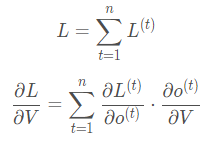
Referring back to the structure diagram, there are three parameters to optimize: W, U, and V. Unlike the BP algorithm, the optimization process for parameters W and U requires tracing back through historical data, while parameter V is relatively straightforward and only needs to focus on the present. Let’s first solve the partial derivative of parameter V.

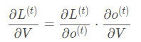
This equation appears simple but is easy to make mistakes because it involves the activation function, which is a composite function requiring differentiation.

The loss of the RNN also accumulates over time, so we cannot only compute the partial derivative at time t.

The partial derivatives of W and U are relatively complex because they need to involve historical data. Let’s assume there are only three time steps; then, at the third time step, the partial derivative of L with respect to W is:

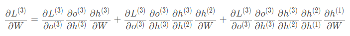
Correspondingly, the partial derivative of L with respect to U at the third time step is:

It can be observed that the partial derivative of L with respect to W or U at a certain time step requires tracing back to all previous time steps, and this is just for one time step’s partial derivative. As mentioned earlier, the loss also accumulates, so the overall partial derivative of the loss function with respect to W and U will be very cumbersome. Nevertheless, the good news is that there are still patterns to follow, and based on the above two equations, we can write the general form of the partial derivative of L with respect to W and U at time t:

The overall partial derivative formula is to sum them up over time.

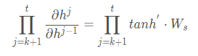
As mentioned earlier, the activation function is nested within, so if we incorporate the activation function and extract the cumulative product:

We find that the cumulative product leads to the derivatives of the activation function being multiplied, which in turn causes gradient vanishing and gradient explosion phenomena.

Gradient Vanishing and Gradient Explosion

Causes

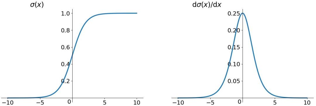
Let’s first look at the graphs of these two activation functions. This is the graph and derivative of the sigmoid function.

This is the graph and derivative of the tanh function.

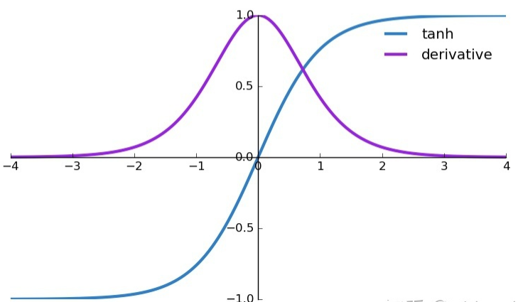
From the above graphs, we can see that when the activation function is the tanh function, the maximum value of its derivative is 1, but it cannot consistently reach 1, which is a rare occurrence. This means that most of the time, the derivatives are less than 1, and when t is very large, the product in h approaches 0, which is the reason for gradient vanishing in RNNs.

You might argue that RNNs are different from deep neural networks; RNN parameters are shared, and the gradient at a certain moment is the accumulation of this moment and previous moments. While this is true, if we use limited gradients to update shared parameters across many layers, issues will inevitably arise, as limited information cannot serve as an optimal solution for all parameters.

Gradient vanishing means that the parameters of that layer will no longer be updated, rendering that hidden layer merely a mapping layer without meaning. Therefore, in deep neural networks, sometimes adding more neurons may be less beneficial than increasing depth.

Next, we look at the equation:

In this equation, W also needs the network parameters U. If the values in the parameter W are too large, and there is a long-term dependency issue with the sequence length, then the problem becomes gradient explosion instead of gradient vanishing. In practical applications, RNNs tend to be deep, making the issues of gradient explosion or gradient vanishing more pronounced.

It was previously mentioned that we often use the tanh function as the activation function; however, the maximum derivative of the tanh function is only 1, and it cannot always reach 1, which means that it is still a bunch of small numbers being multiplied, leading to “gradient vanishing.” So why do we still use it as an activation function? The reason is that the tanh function has a larger gradient compared to the sigmoid function, converges faster, and leads to gradient vanishing more slowly.

Another reason is that the tanh function has a drawback: the sigmoid function output is not zero-centered. The output of the sigmoid is always greater than 0, which means that the output does not have a zero mean, leading to a bias phenomenon. This causes the neurons in the next layer to treat the non-zero mean signal from the previous layer as input. Networks converge better with zero-centered inputs and outputs.

Solutions

The characteristics of RNNs inherently allow for