Source: DeepHub IMBA

This article is about 6800 words, and it is recommended to read for 10+minutes

This article will discuss the techniques to obtain tangible value from the dataset using hypothesis testing, feature engineering, and time series modeling methods.

Using statistical tests and machine learning to analyze and predict the performance of solar power generation.

This article will discuss the techniques to obtain tangible value from the dataset using hypothesis testing, feature engineering, and time series modeling methods. I will also address issues such as data leakage and data preparation in different time series models, and conduct comparative tests on three common time series forecasting methods.

Introduction

Time series forecasting is a frequently studied topic, and we will use data from two solar power plants to model their patterns. First, we will summarize them into two questions to address:

1. Is it possible to identify underperforming solar components?
2. Can we forecast solar power generation for two days?

Before continuing to answer these questions, let us first understand how solar power plants generate electricity.

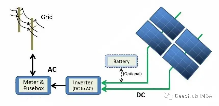
The above figure describes the power generation process from solar panel modules to the grid. Solar energy is directly converted into electrical energy through the photoelectric effect. When materials like silicon (the most common semiconductor material in solar panels) are exposed to light, photons (subatomic particles of electromagnetic energy) are absorbed and release free electrons, generating direct current (DC). Using inverters, DC is converted into alternating current (AC) and sent to the grid, where it can be distributed to homes.

Data

The raw data consists of two comma-separated value (CSV) files for each solar power plant. One file shows the power generation process, and the other file shows the measurement data recorded by the sensors of the solar power plant. Each dataset for the solar power plants is organized into a pandas DataFrame.

The data for Solar Power Plant 1 (SP1) and Solar Power Plant 2 (SP2) is collected every 15 minutes from May 15, 2020, to June 18, 2020. Both SP1 and SP2 datasets contain the same variables.

• Date Time – Interval of 15 minutes
• Ambient temperature – Temperature of the air around the module
• Module temperature – Temperature of the module
• Irradiation – Radiation on the module
• DC Power (kW) – Direct current
• AC Power (kW) – Alternating current
• Daily Yield – Total daily power generation
• Total Yield – Cumulative output of the inverter
• Plant ID – Unique identifier for the solar power plant
• Module ID – Unique identifier for each module

Weather sensors are used to record the ambient temperature, module temperature, and radiation for each solar power plant.

For this dataset, DC power will be the dependent variable (target variable). Our goal is to identify underperforming solar modules.

Two separate DataFrames are used for analysis and prediction. The only difference is that the data used for prediction is resampled to hourly intervals, while the analysis DataFrame contains 15-minute intervals.

First, we remove the Plant ID as it has no value in trying to answer the above questions. The Module ID is also removed from the prediction dataset. Tables 1 and 2 show sample data.

Before continuing to analyze the data, we made some assumptions about the solar power plants, including:

• Data collection instruments are fault-free;
• Modules are regularly cleaned (ignoring maintenance impacts);

• There are no shading issues around both solar power plants.

Exploratory Data Analysis (EDA)

For beginners in data science, EDA is a crucial step to understanding the data through visualization and performing statistical tests. We first observe the performance of each solar power plant by plotting the DC and AC of SP1 and SP2.

SP1 shows that the DC power is an order of magnitude higher than SP2. Assuming the data collected by SP1 is correct and the instruments used to record the data are fault-free, it indicates that the inverter in SP1 needs further investigation.

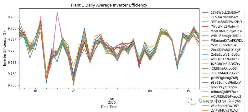
By aggregating the AC and DC power on a daily frequency for each module, Figure 3 shows the inverter efficiency of all modules in SP1. According to industry knowledge, the efficiency of solar inverters should be between 93-96%. Since the efficiency of all modules ranges from 9.76% – 9.79%, it indicates a need to investigate the performance of the inverter and whether it needs replacement.

Since SP1 shows issues with the inverter, further analysis was conducted only on SP2.

Although this brief analysis took more of our time to investigate the inverter, it did not address the main question of identifying the performance of the solar modules.

Since the inverter in SP2 is functioning normally, we can identify and investigate any anomalies by digging deeper into the data.

Figure 4 shows the relationship between module temperature and ambient temperature, with some modules exhibiting extremely high temperatures.

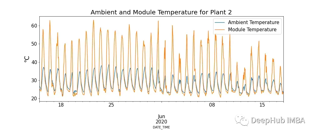
This seems to contradict our understanding, but it is evident that high temperatures negatively affect solar panels. When photons interact with electrons in the solar cell, they release free electrons, but at higher temperatures, more electrons are already in an excited state, which reduces the voltage the panel can produce, thus lowering efficiency.

Considering this phenomenon, the following Figure 5 shows the module temperature and DC power of SP2 (data points where the ambient temperature is lower than the module temperature and times during a day with fewer modules operating have been filtered to prevent data skew).

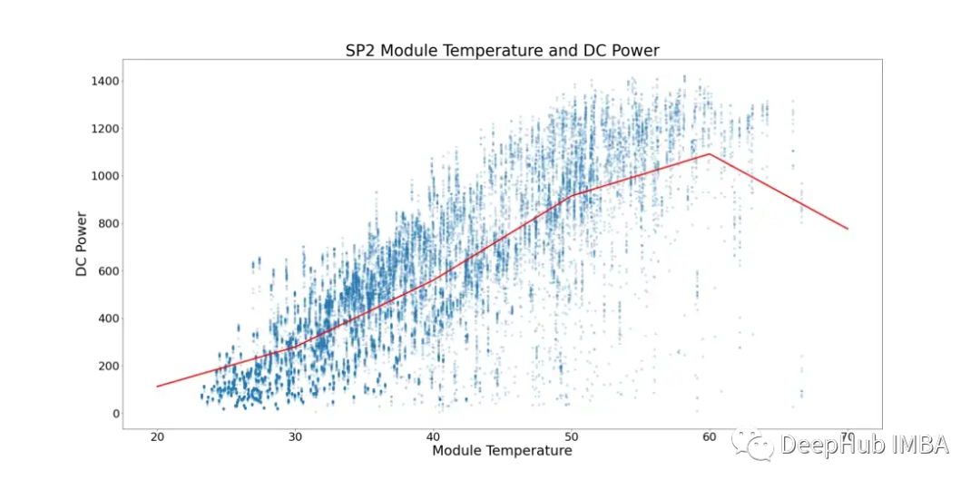
In Figure 5, the red line represents the average temperature. Here, we can see a clear critical point and signs of stagnation in DC power. It starts to plateau at ~52°C. To find the underperforming solar modules, all rows showing module temperatures above 52°C have been removed.

The following Figure 6 shows the DC power of each module in SP2 over a day. This generally aligns with expectations, as power generation is higher at noon. However, there is an issue where power generation is lower during peak operating times. We find it challenging to summarize the reasons for this, as weather conditions on that day may have been poor, or SP2 may require routine maintenance, etc.

Figure 6 also indicates signs of low-performing modules. They can be identified as modules (individual data points) that deviate from the most recent clusters on the graph.

To determine which modules are underperforming, we can perform statistical tests while comparing the performance of each module with others to ascertain performance.

The distribution of DC power from different modules every 15 minutes is normally distributed, and hypothesis testing can identify which modules are underperforming. The count refers to the number of times a module falls outside the 99.9% confidence interval with a p-value < 0.001.

Figure 7 displays the number of times each module is statistically significantly lower than other modules during the same period in descending order.

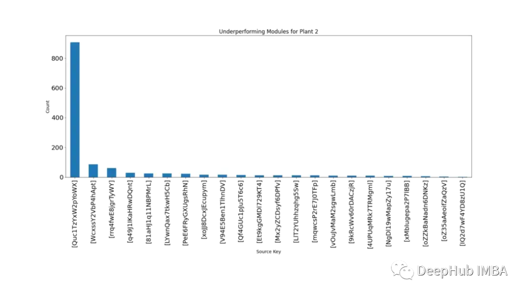
From Figure 7, it is clear that the module ‘Quc1TzYxW2pYoWX’ is problematic. This information can be provided to the relevant personnel at SP2 for investigation.

Modeling

Next, we will start modeling using three different time series algorithms: SARIMA, XGBoost, and CNN-LSTM, and compare them.

For all three models, we will predict the next data point. Walk-forward validation is a technique used for time series modeling because predictions become less accurate over time, so a more practical approach is to retrain the model with actual data as it becomes available.

Before modeling, we need to study the data in more detail. Figure 8 shows the correlation heatmap of all features in the SP2 dataset. The heatmap demonstrates a strong correlation between the dependent variable DC power and the module temperature, irradiation, and ambient temperature. These features may play a crucial role in the predictions.

In the heatmap below, AC power shows a Pearson correlation coefficient of 1. To prevent data leakage issues, we will remove DC power from the data.

SARIMA

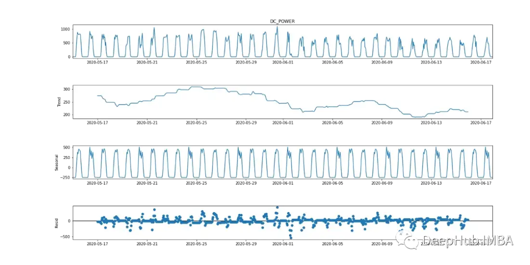
Seasonal Autoregressive Integrated Moving Average (SARIMA) is a univariate time series forecasting method. Since the target variable shows signs of a 24-hour cyclic period, SARIMA is an effective modeling option as it accounts for seasonal effects. This can be observed in the seasonal decomposition plot below.

The SARIMA algorithm requires the data to be stationary. There are various methods to test if the data is stationary, such as statistical tests (Augmented Dickey-Fuller test), summary statistics (comparing means/variances of different parts of the data), and visual analysis of the data. It is important to conduct multiple tests before modeling.

The Augmented Dickey-Fuller (ADF) test is a “unit root test” used to determine if a time series is stationary. Essentially, this is a statistical significance test where there is a null hypothesis and an alternative hypothesis, and conclusions are drawn based on the resulting p-value.

Null Hypothesis: The time series data is non-stationary.

Alternative Hypothesis: The time series data is stationary.

In our case, if the p-value ≤ 0.05, we can reject the null hypothesis and confirm that the data has no unit root.

from statsmodels.tsa.stattools import adfuller
result = adfuller(plant2_dcpower.values)
print('ADF Statistic: %f' % result[0])
print('p-value: %f' % result[1])
print('Critical Values:')
for key, value in result[4].items():
    print('\t%s: %.3f' % (key, value))

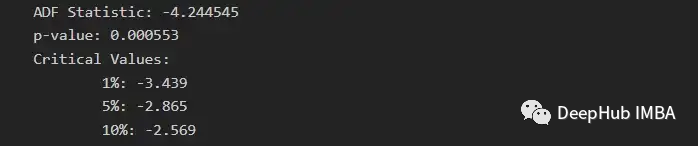
From the ADF test, the p-value is 0.000553, < 0.05. Based on this statistical data, it can be concluded that the data is stable. However, looking at Figure 2 (the topmost figure), there are evident seasonal signs (for time series data deemed stationary, there should be no signs of seasonality or trends), indicating that the data is non-stationary. Therefore, running multiple tests is very important.

To model the dependent variable using SARIMA, the time series needs to be stationary. As shown in Figure 9 (the first and third graphs), DC power exhibits obvious seasonal signs. Taking the first difference [t-(t-1)] removes the seasonal component, as shown in Figure 10, because it appears similar to a normal distribution. The data is now stationary and suitable for the SARIMA algorithm.

The hyperparameters of SARIMA include p (autoregressive order), d (degree of differencing), q (moving average order), P (seasonal autoregressive order), D (seasonal differencing order), Q (seasonal moving average order), m (time steps of seasonal period), trend (deterministic trend).

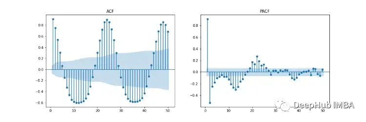
Figure 11 shows the autocorrelation (ACF), partial autocorrelation (PACF), and seasonal ACF/PACF plots. The ACF plot shows the correlation between the time series and its lagged versions. The PACF shows the direct correlation between the time series and its lagged versions. The blue shaded area represents the confidence interval. SACF and SPACF can be calculated by taking seasonal differences (m) from the original data, which in this case is 24, as there is an evident 24-hour seasonal effect in the ACF plot.

According to our intuition, the starting point for hyperparameters can be derived from the ACF and PACF plots. If both ACF and PACF show a gradually declining trend, both the autoregressive order (p) and the moving average order (q) are greater than 0. p and P can be determined by observing the PCF and SPCF plots, respectively, and calculating the number of lags that are statistically significant before they become insignificant. Similarly, q and Q can be found in the ACF and SACF plots.

The degree of differencing (d) can be determined by the number of differences required to make the data stationary. The seasonal differencing degree (D) is estimated based on the number of differences needed to remove the seasonal component from the time series.

These hyperparameter selections can be found in this article: https://arauto.readthedocs.io/en/latest/how_to_choose_terms.html

A grid search method can also be used for hyperparameter optimization, selecting the optimal hyperparameters based on the minimum mean squared error (MSE), including p = 2, d = 0, q = 4, P = 2, D = 1, Q = 6, m = 24, trend = ‘n’ (no trend).

from time import time
from sklearn.metrics import mean_squared_error
from statsmodels.tsa.statespace.sarimax import SARIMAX

configg = [(2, 1, 4), (2, 1, 6, 24), 'n']

def train_test_split(data, test_len=48):
    """
    Split data into training and testing.
    """
    train, test = data[:-test_len], data[-test_len:]
    return train, test

def sarima_model(data, cfg, test_len, i):
    """
    SARIMA model which outputs prediction and model.
    """
    order, s_order, t = cfg[0], cfg[1], cfg[2]
    model = SARIMAX(data, order=order, seasonal_order=s_order, trend=t,
                     enforce_stationarity=False, enforce_invertibility=False)
    model_fit = model.fit(disp=False)
    yhat = model_fit.predict(len(data))
    if i + 1 == test_len:
        return yhat, model_fit
    else:
        return yhat

def walk_forward_val(data, cfg):
    """
    A walk forward validation technique used for time series data. Takes current value of x_test and predicts
    value. x_test is then fed back into history for the next prediction.
    """
    train, test = train_test_split(data)
    pred = []
    history = [i for i in train]
    test_len = len(test)
    for i in range(test_len):
        if i + 1 == test_len:
            yhat, s_model = sarima_model(history, cfg, test_len, i)
            pred.append(yhat)
            mse = mean_squared_error(test, pred)
            return pred, mse, s_model
        else:
            yhat = sarima_model(history, cfg, test_len, i)
            pred.append(yhat)
            history.append(test[i])
    pass

if __name__ == '__main__':
    start_time = time()
    sarima_pred_plant2, sarima_mse, s_model = walk_forward_val(plant2_dcpower, configg)
    time_len = time() - start_time
    print(f'SARIMA runtime: {round(time_len/60,2)} mins')

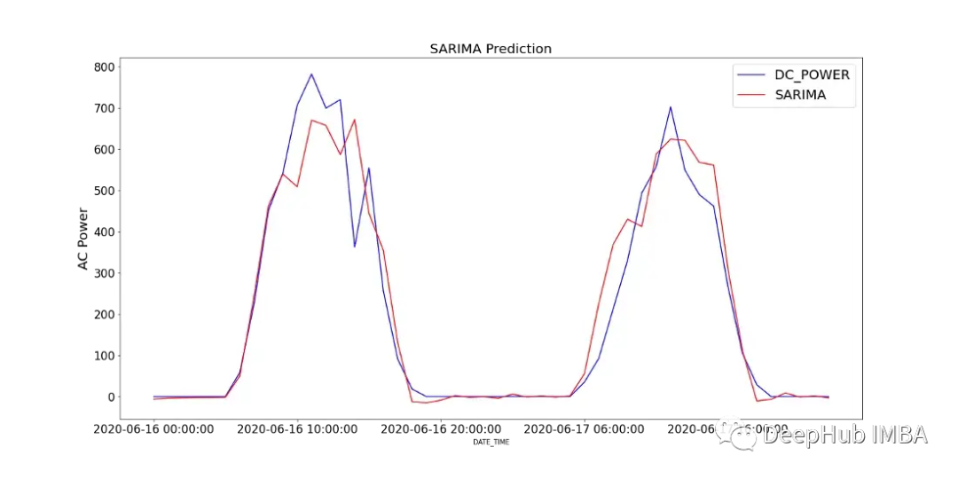
Figure 12 shows a comparison of the predicted values of the SARIMA model with the recorded DC power of SP2 over two days.

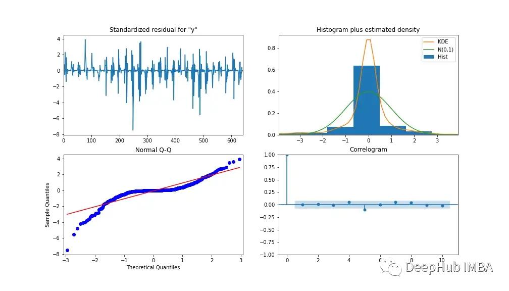
To analyze the performance of the model, Figure 13 shows the model diagnostics. The relevant plots show nearly no correlation after the first lag, and the histogram below shows a normal distribution around a mean of zero. Thus, we can say that the model is unable to gather further information from the data.

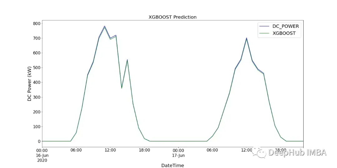
XGBoost

XGBoost (eXtreme Gradient Boosting) is a gradient-boosted decision tree algorithm. It uses an ensemble method where new decision tree models are added to modify existing decision tree scores. Unlike SARIMA, XGBoost is a multivariate machine learning algorithm, meaning that this model can take multiple features to enhance performance.

We use feature engineering to improve model accuracy. Three additional features are created, including lagged versions of AC and DC power, referred to as S1_AC_POWER and S1_DC_POWER, respectively, and overall efficiency EFF calculated as AC_POWER divided by DC_POWER. We also remove AC_POWER and MODULE_TEMPERATURE from the data. Figure 14 shows the importance levels of features through gain (average gain of splits using one feature) and weight (the number of times a feature appears in trees).

Hyperparameters used for modeling were determined through grid search, resulting in: *learning rate = 0.01, number of estimators = 1200, subsample = 0.8, colsample by tree = 1, colsample by level = 1, min child weight = 20 and max depth = 10

We use MinMaxScaler to scale the training data between 0 and 1 (other scalers like log-transform and standard-scaler can also be experimented with depending on the data distribution). By shifting all independent variables back in time, we convert the data into a supervised learning dataset.

import numpy as np
import pandas as pd
import xgboost as xgb
from sklearn.preprocessing import MinMaxScaler
from time import time

def train_test_split(df, test_len=48):
    """
    split data into training and testing.
    """
    train, test = df[:-test_len], df[-test_len:]
    return train, test

def data_to_supervised(df, shift_by=1, target_var='DC_POWER'):
    """
    Convert data into a supervised learning problem.
    """
    target = df[target_var][shift_by:].values
    dep = df.drop(target_var, axis=1).shift(-shift_by).dropna().values
    data = np.column_stack((dep, target))
    return data

def xgb_forecast(train, x_test):
    """
    XGBOOST model which outputs prediction and model.
    """
    x_train, y_train = train[:,:-1], train[:,-1]
    xgb_model = xgb.XGBRegressor(learning_rate=0.01, n_estimators=1500,
                                  subsample=0.8, colsample_bytree=1,
                                  colsample_bylevel=1, min_child_weight=20,
                                  max_depth=14, objective='reg:squarederror')
    xgb_model.fit(x_train, y_train)
    yhat = xgb_model.predict([x_test])
    return yhat[0], xgb_model

def walk_forward_validation(df):
    """
    A walk forward validation approach by scaling the data and changing into a supervised learning problem.
    """
    preds = []
    train, test = train_test_split(df)
    scaler = MinMaxScaler(feature_range=(0,1))
    train_scaled = scaler.fit_transform(train)
    test_scaled = scaler.transform(test)
    train_scaled_df = pd.DataFrame(train_scaled, columns = train.columns, index=train.index)
    test_scaled_df = pd.DataFrame(test_scaled, columns = test.columns, index=test.index)
    train_scaled_sup, test_scaled_sup = data_to_supervised(train_scaled_df), data_to_supervised(test_scaled_df)
    history = np.array([x for x in train_scaled_sup])
    for i in range(len(test_scaled_sup)):
        test_x, test_y = test_scaled_sup[i][:-1], test_scaled_sup[i][-1]
        yhat, xgb_model = xgb_forecast(history, test_x)
        preds.append(yhat)
        np.append(history,[test_scaled_sup[i]], axis=0)
    pred_array = test_scaled_df.drop("DC_POWER", axis=1).to_numpy()
    pred_num = np.array([pred])
    pred_array = np.concatenate((pred_array, pred_num.T), axis=1)
    result = scaler.inverse_transform(pred_array)
    return result, test, xgb_model

if __name__ == '__main__':
    start_time = time()
    xgb_pred, actual, xgb_model = walk_forward_validation(dropped_df_cat)
    time_len = time() - start_time
    print(f'XGBOOST runtime: {round(time_len/60,2)} mins')

Figure 15 shows a comparison of the predicted values of the XGBoost model with the recorded DC power of SP2 over two days.

CNN-LSTM

CNN-LSTM (Convolutional Neural Network Long-Short-Term Memory) is a hybrid model of two neural network models. CNN is a feedforward neural network that has shown good performance in image processing and natural language processing. It can also be effectively applied to forecasting time series data. LSTM is a sequence-to-sequence neural network model designed to address the long-standing issues of gradient explosion/vanishing, using an internal memory system that allows it to accumulate states over input sequences.

In this case, CNN-LSTM is used as an encoder-decoder architecture. Since CNN does not directly support sequence input, we read the sequence input through a 1D CNN and automatically learn important features. The LSTM then performs the decoding. Similar to the XGBoost model, we use the same data and scale it using scikit-learn’s MinMaxScaler, but the range is between -1 and 1. For CNN-LSTM, the data needs to be reshaped into the required structure: [samples, subsequences, timesteps, features] so that it can be passed as input to the model.

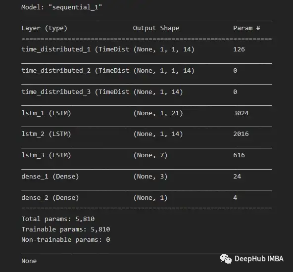
Since we want to reuse the same CNN model for each subsequence, we apply the entire model once to each input subsequence using TimeDistributedWrapper. In the following Figure 16, the model summary shows the different layers used in the final model.

After splitting the data into training and testing datasets, the training data is further divided into training and validation datasets. After each iteration with all training data (including validation data), the model can further use this to evaluate its performance.

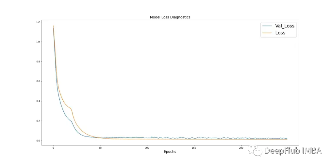
Learning curves are a great diagnostic tool used in deep learning, showing how the model performs after each stage. The following Figure 17 shows how the model learns from the data and displays the convergence of validation data with training data. This is a sign of good model training.

import pandas as pd
import numpy as np
from sklearn.metrics import mean_squared_error
from sklearn.preprocessing import MinMaxScaler
import keras
from keras.models import Sequential
from keras.layers.convolutional import Conv1D, MaxPooling1D
from keras.layers import LSTM, TimeDistributed, RepeatVector, Dense, Flatten
from keras.optimizers import Adam

n_steps = 1
subseq = 1

def train_test_split(df, test_len=48):
    """
    Split data in training and testing. Use 48 hours as testing.
    """
    train, test = df[:-test_len], df[-test_len:]
    return train, test

def split_data(sequences, n_steps):
    """
    Preprocess data returning two arrays.
    """
    x, y = [], []
    for i in range(len(sequences)):
        end_x = i + n_steps
        if end_x > len(sequences):
            break
        x.append(sequences[i:end_x, :-1])
        y.append(sequences[end_x-1, -1])
    return np.array(x), np.array(y)


def CNN_LSTM(x, y, x_val, y_val):
    """
    CNN-LSTM model.
    """
    model = Sequential()
    model.add(TimeDistributed(Conv1D(filters=14, kernel_size=1, activation="sigmoid",
                                      input_shape=(None, x.shape[2], x.shape[3]))))
    model.add(TimeDistributed(MaxPooling1D(pool_size=1)))
    model.add(TimeDistributed(Flatten()))
    model.add(LSTM(21, activation="tanh", return_sequences=True))
    model.add(LSTM(14, activation="tanh", return_sequences=True))
    model.add(LSTM(7, activation="tanh"))
    model.add(Dense(3, activation="sigmoid"))
    model.add(Dense(1))
    model.compile(optimizer=Adam(learning_rate=0.001), loss="mse", metrics=['mse'])
    history = model.fit(x, y, epochs=250, batch_size=36,
                        verbose=0, validation_data=(x_val, y_val))
    return model, history

# split and reshape data
train, test = train_test_split(dropped_df_cat)
train_x = train.drop(columns="DC_POWER", axis=1).to_numpy()
train_y = train["DC_POWER"].to_numpy().reshape(len(train), 1)
test_x = test.drop(columns="DC_POWER", axis=1).to_numpy()
test_y = test["DC_POWER"].to_numpy().reshape(len(test), 1)

# scale data
scaler_x = MinMaxScaler(feature_range=(-1,1))
scaler_y = MinMaxScaler(feature_range=(-1,1))
train_x = scaler_x.fit_transform(train_x)
train_y = scaler_y.fit_transform(train_y)
test_x = scaler_x.transform(test_x)
test_y = scaler_y.transform(test_y)

# shape data into CNN-LSTM format [samples, subsequences, timesteps, features]
ORIGINAL train_data_np = np.hstack((train_x, train_y))
x, y = split_data(train_data_np, n_steps)
x_subseq = x.reshape(x.shape[0], subseq, x.shape[1], x.shape[2])

# create validation set
x_val, y_val = x_subseq[-24:], y[-24:]
x_train, y_train = x_subseq[:-24], y[:-24]
n_features = x.shape[2]
actual = scaler_y.inverse_transform(test_y)

# run CNN-LSTM model
if __name__ == '__main__':
    start_time = time()
    model, history = CNN_LSTM(x_train, y_train, x_val, y_val)
    prediction = []
    for i in range(len(test_x)):
        test_input = test_x[i].reshape(1, subseq, n_steps, n_features)
        yhat = model.predict(test_input, verbose=0)
        yhat_IT = scaler_y.inverse_transform(yhat)
        prediction.append(yhat_IT[0][0])
    time_len = time() - start_time
    mse = mean_squared_error(actual.flatten(), prediction)
    print(f'CNN-LSTM runtime: {round(time_len/60,2)} mins')
    print(f"CNN-LSTM MSE: {round(mse,2)}")

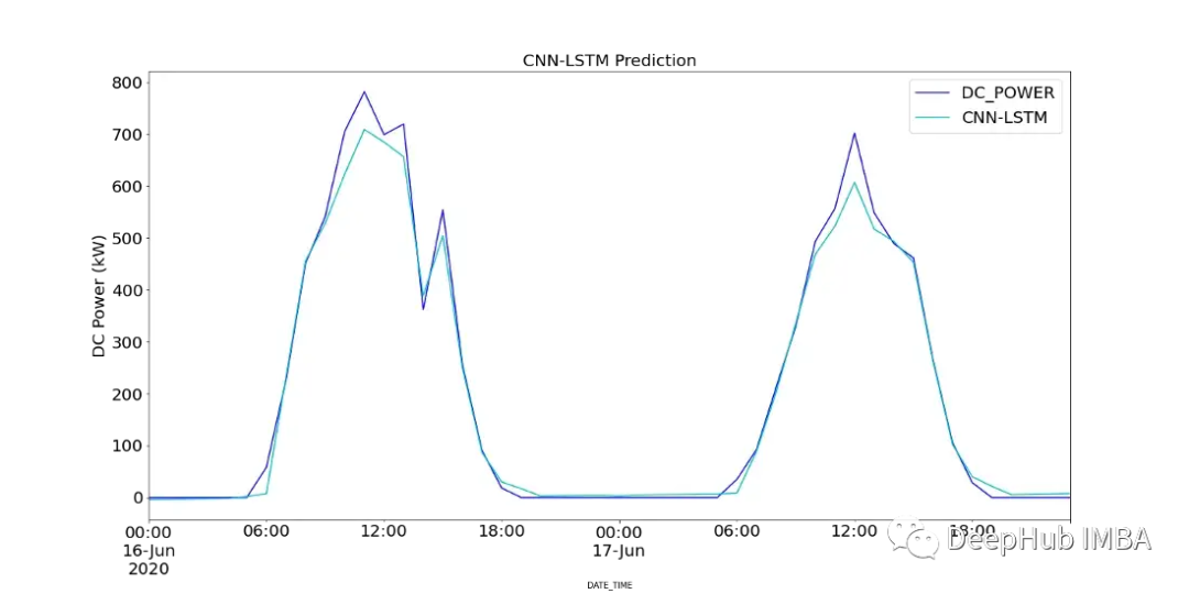
Figure 18 shows a comparison of the predicted values of the CNN-LSTM model with the recorded DC power of SP2 over two days.

Due to the randomness of CNN-LSTM, the model was run 10 times, and an average MSE value was recorded as the final value to assess model performance. Figure 19 shows the range of MSE recorded for all models.

Results Comparison

The table below shows the MSE of each model (average MSE for CNN-LSTM) and the runtime of each model (in minutes).

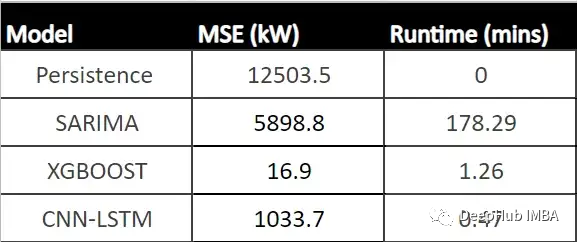
From the table, it can be seen that XGBoost has the lowest MSE, the second-fastest runtime, and exhibits the best performance compared to all other models. Since this model shows an acceptable runtime for hourly predictions, it can serve as a powerful tool to aid the decision-making process for operations managers.

Conclusion

In this article, we analyzed SP1 and SP2, identifying that SP1 has lower performance. Further investigation of SP2 showed which modules may have performance issues, and we used hypothesis testing to calculate the number of times each module significantly underperformed statistically, with the ‘Quc1TzYxW2pYoWX’ module showing about 850 counts of low performance.

We trained three models using the data: SARIMA, XGBoost, and CNN-LSTM. SARIMA performed the worst, while XGBOOST performed the best with an MSE of 16.9 and a runtime of 1.43 minutes. Thus, it can be said that XGBoost is the optimal choice in tabular data.

Article Code: https://github.com/Amitdb123/Solar_Power_Analysis-Prediction

Dataset: https://www.kaggle.com/datasets/ef9660b4985471a8797501c8970009f36c5b3515213e2676cf40f540f0100e54

Author: Amit Bharadwa

Editor: Huang Jiyan