Introduction


The original official tutorial URL: https://juliasilge.com/blog/xgboost-tune-volleyball/
Notes
-
1. Due to poor external data currently, the data used is the test data from the tidytuesdayR package. -
2. Tidymodels is an integrated R language machine learning environment developed by the R Studio team, with a unified interface and results which facilitate subsequent benchmark analysis. -
3. The tidymodels system has good support for classification and regression tasks, and the syntax is quite similar to the tidyverse flow, making it easy to get started; however, its support for survival data is relatively poor. -
4. Divide the dataset – determine the model – adjust hyperparameters – apply the model (breaking down complex model problems into methodological problems akin to putting an elephant in a refrigerator).
Code Example
## Load required R packages
rm(list = ls())
options(stringsAsFactors = T)

library(tidyverse)
library(tidymodels)
library(tidytuesdayR)
library(doParallel)
library(vip)

# Load dataset
tuesdata <- tidytuesdayR::tt_load('2020-05-19')
vb_matches <- tuesdata$vb_matches

# Select variables to rebuild the dataset
vb_parsed <- vb_matches %>%
  transmute(
    circuit,
    gender,
    year,
    w_attacks = w_p1_tot_attacks + w_p2_tot_attacks,
    w_kills = w_p1_tot_kills + w_p2_tot_kills,
    w_errors = w_p1_tot_errors + w_p2_tot_errors,
    w_aces = w_p1_tot_aces + w_p2_tot_aces,
    w_serve_errors = w_p1_tot_serve_errors + w_p2_tot_aces,
    w_blocks = w_p1_tot_blocks + w_p2_tot_blocks,
    w_digs = w_p1_tot_digs + w_p2_tot_digs,
    l_attacks = l_p1_tot_attacks + l_p2_tot_attacks,
    l_kills = l_p1_tot_kills + l_p2_tot_kills,
    l_errors = l_p1_tot_errors + l_p2_tot_errors,
    l_aces = l_p1_tot_aces + l_p2_tot_aces,
    l_serve_errors = l_p1_tot_serve_errors + l_p2_tot_aces,
    l_blocks = l_p1_tot_blocks + l_p2_tot_blocks,
    l_digs = l_p1_tot_digs + l_p2_tot_digs
  ) %>%
  na.omit()

# Construct binary classification outcome variable
winners <- vb_parsed %>%
  select(circuit, gender, year,
         w_attacks:w_digs) %>% # Can filter variables by column name order
  rename_with(~ str_remove_all(., "w_"), w_attacks:w_digs) %>%
  mutate(win = "win")

losers <- vb_parsed %>%
  select(circuit, gender, year,
         l_attacks:l_digs) %>%
  rename_with(~ str_remove_all(., "l_"), l_attacks:l_digs) %>%
  mutate(win = "lose")

vb_df <- bind_rows(winners, losers) %>%
  mutate_if(is.character, factor)
# Construct training and testing sets
set.seed(2022)
# Reduce dataset size for faster computation
vb_df %>%
initial_split(strata = win, prop = 0.1) %>%
training() -> vb_df
# Split into training and testing sets
vb_split <- initial_split(vb_df, strata = win)
vb_train <- training(vb_split)
vb_test <- testing(vb_split)
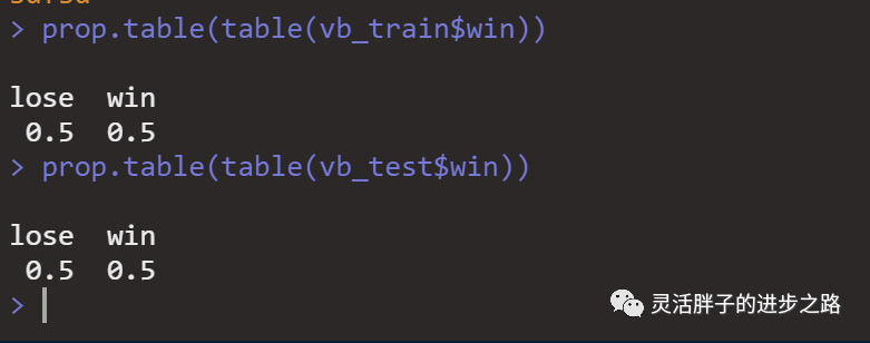
# View distribution ratio
prop.table(table(vb_train$win))
prop.table(table(vb_test$win))
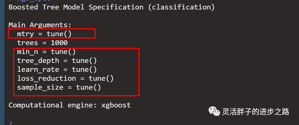
# Construct model and determine hyperparameters to adjust
xgb_spec <- boost_tree(
trees = 1000,
tree_depth = tune(), min_n = tune(),
loss_reduction = tune(), ## first three: model complexity
sample_size = tune(), mtry = tune(), ## randomness
learn_rate = tune(), ## step size
) %>%
set_engine("xgboost") %>%
set_mode("classification")
xgb_spec
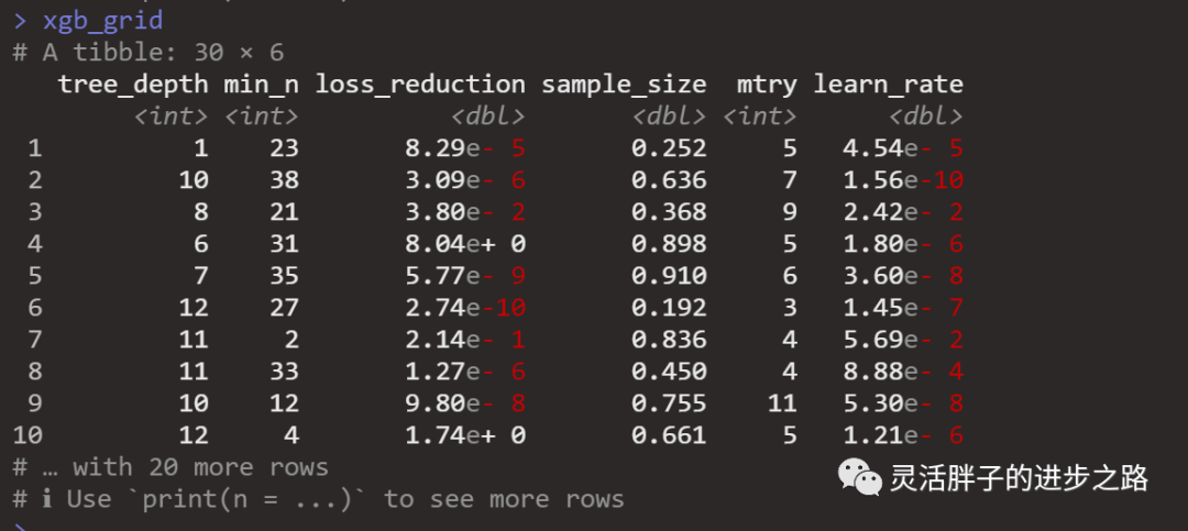
## Determine hyperparameter search scheme
set.seed(2022)
xgb_grid <- grid_latin_hypercube(
tree_depth(),
min_n(),
loss_reduction(),
sample_size = sample_prop(),
finalize(mtry(), vb_train),
learn_rate(),
size = 30
)
xgb_grid
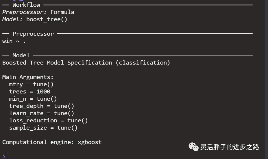
## Create workflow
xgb_wf <- workflow() %>%
add_formula(win ~ .) %>%
add_model(xgb_spec)
xgb_wf
## Determine resampling strategy
set.seed(2022)
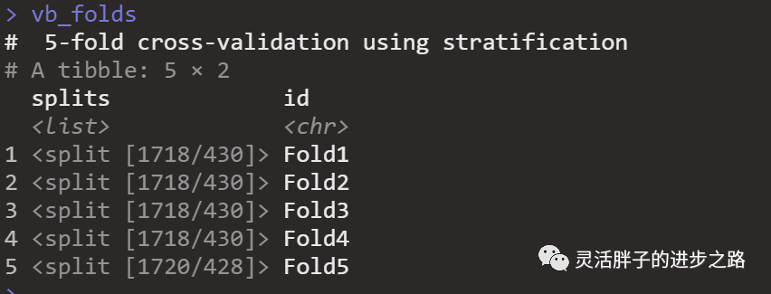
vb_folds <- vfold_cv(vb_train,
strata = win, v = 5)
vb_folds
n_cores <- detectCores() # Determine the number of local machine cores
doParallel::registerDoParallel(n_cores/2) # Use all cores to speed up computation
set.seed(2022)
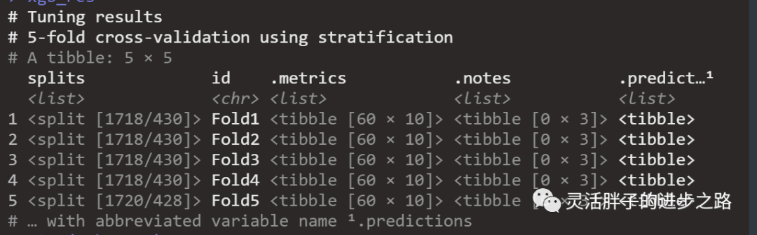
xgb_res <- tune_grid(
xgb_wf, # Workflow
resamples = vb_folds, # Resampling strategy
grid = xgb_grid, # Hyperparameter strategy
control = control_grid(save_pred = TRUE) # Save each hyperparameter result
)
xgb_res
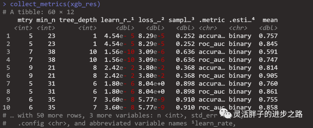
# Commonly check model fitting results
collect_metrics(xgb_res)
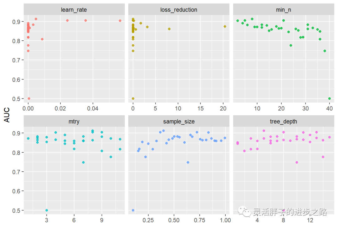
# Plot to show AUC and hyperparameter relationships
xgb_res %>%
collect_metrics() %>%
filter(.metric == "roc_auc") %>%
select(mean, mtry:sample_size) %>%
pivot_longer(mtry:sample_size,
values_to = "value",
names_to = "parameter"
) %>%
ggplot(aes(value, mean, color = parameter)) +
geom_point(alpha = 0.8, show.legend = FALSE) +
facet_wrap(~parameter, scales = "free_x") +
labs(x = NULL, y = "AUC")
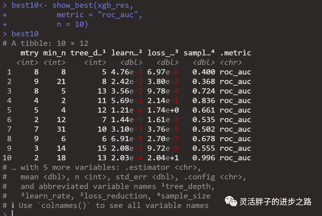
## Show the best model
best10 <- show_best(xgb_res,
metric = "roc_auc",
n = 10)
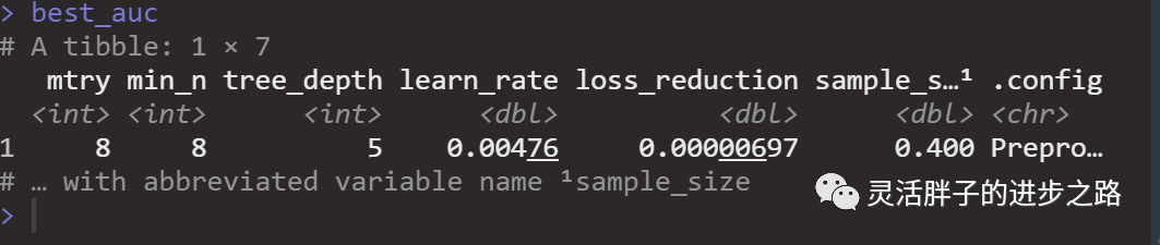
# Select the model with the highest AUC
best_auc <- select_best(xgb_res, "roc_auc")
best_auc
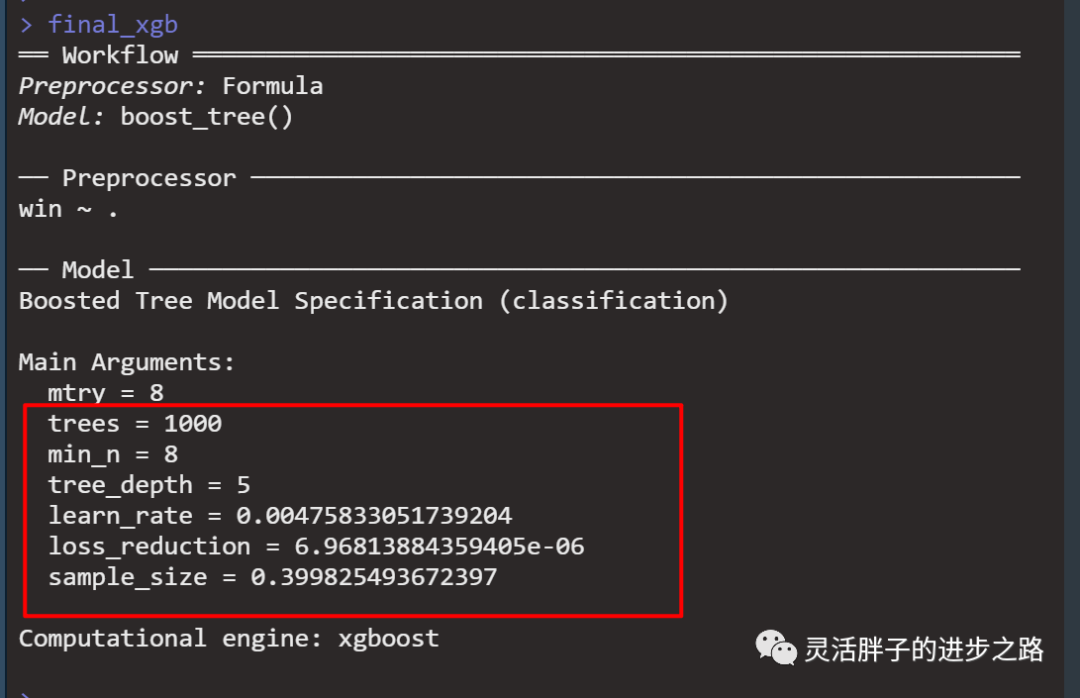
# Final model of the modeling group
final_xgb <- finalize_workflow(
xgb_wf,
best_auc
)
final_xgb
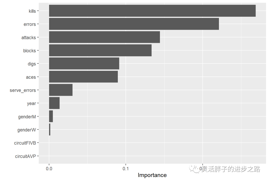
# Use xgboost to determine variable importance
final_xgb %>%
fit(data = vb_train) %>%
extract_fit_parsnip() %>%
vip(geom = "col", num_features = 20)
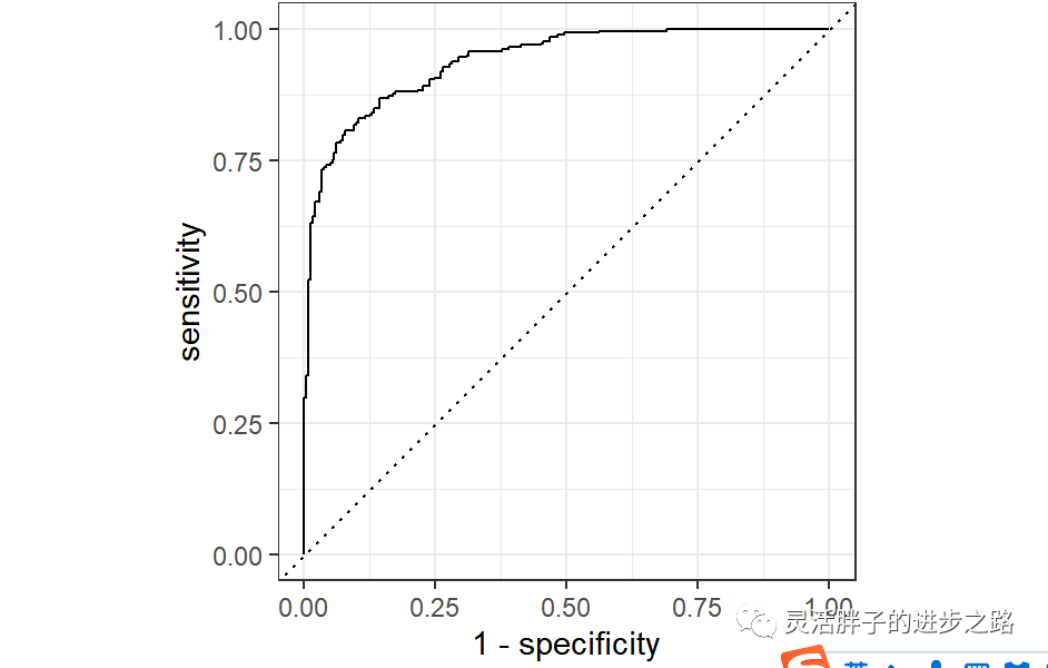
# Fit test set data
final_res <- last_fit(final_xgb, vb_split)
collect_metrics(final_res)
# Draw ROC curve
final_res %>%
collect_predictions() %>%
roc_curve(win, .pred_win) %>%
ggplot(aes(x = 1 - specificity, y = sensitivity)) +
geom_line(size = 1.5, color = "midnightblue") +
geom_abline(
lty = 2, alpha = 0.5,
color = "gray50",
size = 1.2
)
final_xgb %>%
collect_predictions() %>%
roc_curve(win, .pred_win) %>%
ggplot(aes(x = 1 - specificity, y = sensitivity)) +
geom_line(size = 1.5, color = "midnightblue") +
geom_abline(
lty = 2, alpha = 0.5,
color = "gray50",
size = 1.2
)
predict(fit_final, new_data = vb_train)
final_xgb %>%
fit(data = vb_train) -> fit_final