Building and Experimenting with Neural Networks in PyTorch

Author | Tirthajyoti Sarkar

Source | Medium

Editor | Code Doctor Team

Introduction

This article will demonstrate a simple step-by-step process to build a PyTorch 2-layer neural network classifier (fully connected) to illustrate some key features and styles.

PyTorch provides great flexibility for programmers to create, combine, and manipulate tensors as they flow through the network…

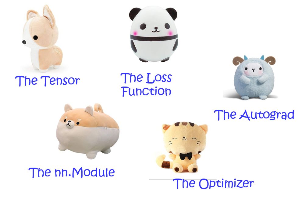
Core Components

The core components of PyTorch used to build a neural classifier are

• Tensors (the central data structure in PyTorch)

• Autograd functionality of Tensors

• nn.Module class for building any other neural class classifiers

• Optimizers

• Loss functions

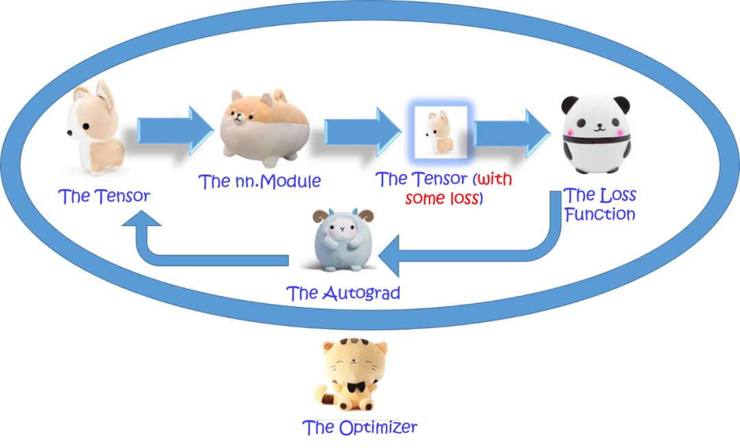
Using these components, we will build a classifier through five simple steps

• Construct the neural network as a custom class (inheriting from nn.Module), which contains hidden layer tensors and a forward method that propagates the input tensor through various layers and activation functions

• Use this forward method to propagate feature tensors (from the dataset) through the network – to get an output tensor

• Calculate the loss by comparing the output against the ground truth, using built-in loss functions

• Backpropagate the gradients of the loss using the automatic differentiation capability (Autograd) with the backward method

• Use the gradients of the loss to update the network’s weights (this is done by performing a step of the so-called optimizer) optimizer.step().

This five-step process constitutes a complete training epoch. Just repeat it to reduce loss and achieve higher classification accuracy.

In PyTorch, defining a neural network as a custom class allows you to reap all the benefits of Object-Oriented programming (OOP) paradigms.

Tensors

torch.Tensor is a multidimensional matrix containing elements of a single data type. It is the central data structure of the framework. You can create a Tensor from Numpy arrays or lists and perform various operations such as indexing, mathematics, and linear algebra.

Tensors support some other enhancements that make them unique. Besides CPU, they can also be loaded onto GPU for faster computations (with just an extremely simple code change). They also support forming a backward graph that tracks every operation applied to them using dynamic computation graphs (DCG) to compute gradients.

Autograd

For complex neural networks, calculus can be quite tricky. High-dimensional spaces can be confusing. Luckily, there is Autograd.

To handle hyperplanes in 14-dimensional space, visualize 3D space and say “fourteen” out loud.

Tensor objects support the magical Autograd functionality of automatic differentiation, which is achieved by tracking and storing all operations performed on Tensors as they flow through the network.

nn.Module Class

In PyTorch, neural networks are built by defining them as custom classes. However, instead of deriving from the original Python object, inherit from the nn.Module class. This injects useful properties and powerful methods into the neural network class. A complete example of this class definition will be seen in this article.

Loss Functions

The loss function defines the distance between the predictions of the neural network and the ground truth, while the quantitative measure of loss helps drive the network closer to the optimal configuration for classifying the given dataset.

PyTorch provides all common loss functions for classification and regression tasks

• Binary and multi-class cross-entropy,

• Mean squared and mean absolute errors

• Smooth L1 loss

• Neg log-likelihood loss

• Kullback-Leibler divergence

Optimizers

Optimizing weights for minimal loss is at the core of the backpropagation algorithm used to train neural networks. PyTorch provides a wide range of optimizers to accomplish this, which are exposed through the torch.optim module.

• Stochastic Gradient Descent (SGD),

• Adam, Adadelta, Adagrad, SparseAdam,

• L-BFGS,

• RMSprop

“The five-step process constitutes a complete training epoch. Just repeat it.”

Neural Network Class and Training

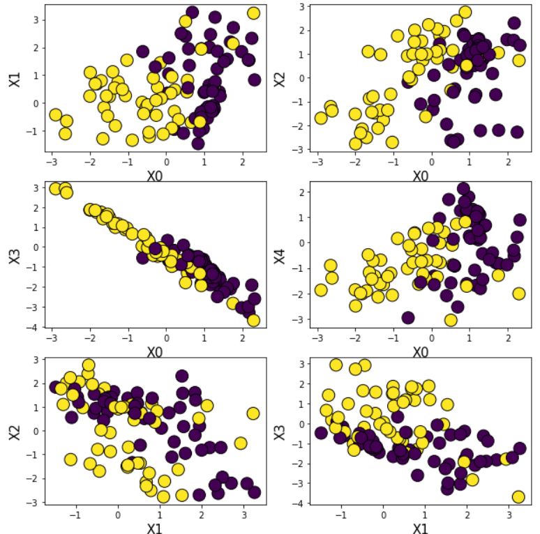
Data

For this example task, we first create some synthetic data using a binary class function from Scikit-learn. In the following chart, data categories are distinguished by color. Clearly, the dataset cannot be separated by a simple linear classifier, and a neural network is a suitable machine learning tool to solve this problem.

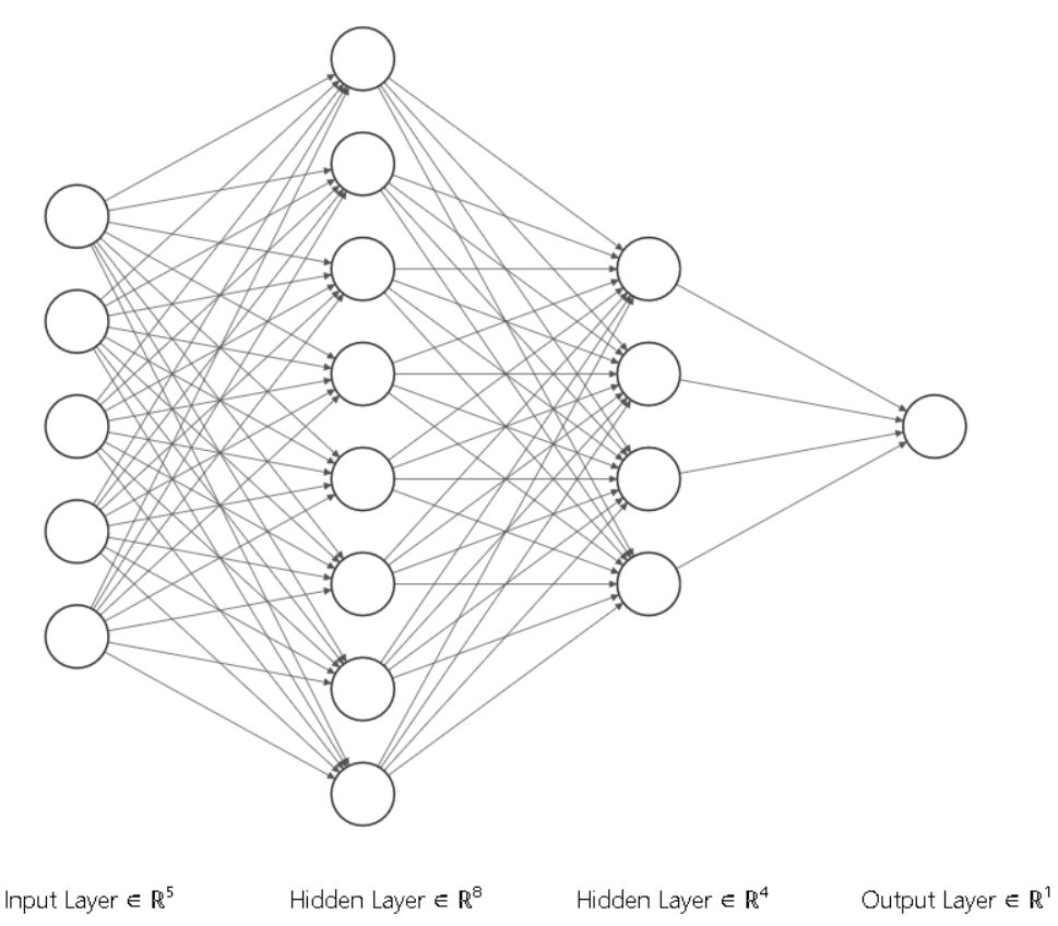
Architecture

A simple fully connected 2 hidden layer architecture was chosen. As shown in the figure below

Class Definition

n_input = X.shape[1] # Must match the shape of the input features
n_hidden1 = 8 # Number of neurons in the 1st hidden layer
n_hidden2 = 4 # Number of neurons in the 2nd hidden layer
n_output = 1 # Number of output units (for example 1 for binary classification)

Define variables corresponding to this architecture, then define the main class. The neural network class is defined as shown below. As mentioned earlier, it inherits from the nn.Module base class.

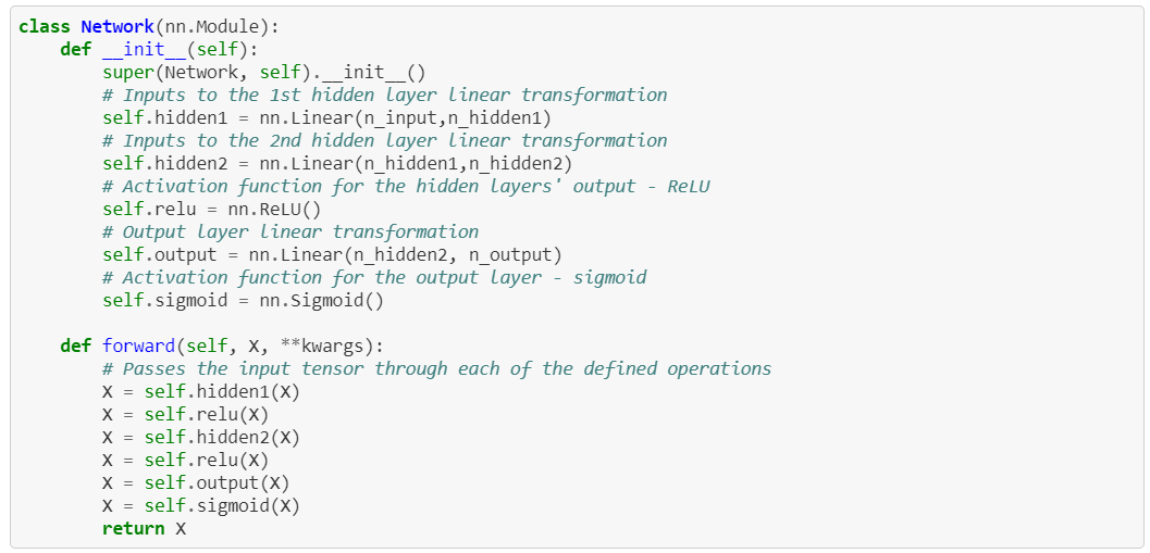
This code has minimal explanation, with added comments. In the method definitions, forward, there is a strong similarity to how Keras defines models.

Also, note the use of built-in linear algebra operations nn.Linear (as between layers) and activation functions (such as nn.ReLU and nn.Sigmoid at the outputs of various layers).

If you instantiate a model object and print it, you will see the structure (parallel to Keras’s model.summary() method).

model = Network()
print(model) # Network(
#   (hidden1): Linear(in_features=5, out_features=8, bias=True)
#   (hidden2): Linear(in_features=8, out_features=4, bias=True)
#   (relu): ReLU()
#   (output): Linear(in_features=4, out_features=1, bias=True)
#   (sigmoid): Sigmoid())

Loss Function, Optimizer, and Training

For this task, we choose binary cross-entropy loss and define it as follows (by convention, the loss function is often called criterion in PyTorch)

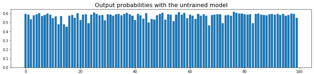
criterion = nn.BCELoss() # Binary cross-entropy loss

At this point, run the input dataset through the defined neural network model, i.e., a forward pass and calculate the output probabilities. Since the weights are initialized randomly, you will see random output probabilities (mostly close to 0.5).

logits = model.forward(X) # Output of the forward pass (logits i.e. probabilities)

If you print the first 10 probabilities, you will get something like this,

tensor([[0.5926],[0.5854],[0.5369],[0.5802],[0.5905],[0.6010],[0.5723],[0.5842],[0.5971],[0.5883]], grad_fn=<SliceBackward>)

All output probabilities appear to be close to 0.5,

Calculating the average loss is straightforward,

loss = criterion(logits,y)

For the optimizer, we choose simple stochastic gradient descent (SGD) and specify the learning rate as 0.1,

from torch import optim
optimizer = optim.SGD(model.parameters(),lr=0.1)

Now we proceed with training. Again, we follow the five steps

• Reset the gradients to zero (to prevent gradient accumulation)

• Pass the tensor forward through the layers

• Calculate the loss tensor

• Calculate the gradients of the loss

• Update the weights by stepping the optimizer (along the direction of the negative gradient)

Surprisingly, if you read the five steps above, this is exactly what you see in all theoretical discussions of neural networks (and all textbooks). And with PyTorch, you can implement this process step by step using seemingly simple code.

Nothing is hidden or abstract. You will feel the raw power and excitement of implementing the neural network training process in five lines of Python code!

# Resets the gradients i.e. do not accumulate over passes
optimizer.zero_grad()
# Forward pass
output = model.forward(X)
# Calculate loss
loss = criterion(output,y)
# Backward pass (AutoGrad)
loss.backward()
# One step of the optimizer
optimizer.step()

Training Multiple Epochs

That was just one epoch. Now it is clear that one epoch won’t cut it, right? To run multiple epochs, just use a loop.

epochs = 10
for i,e in enumerate(range(epochs)):
    optimizer.zero_grad() # Reset the grads
    output = model.forward(X) # Forward pass
    loss = criterion(output.view(output.shape[0]),y) # Calculate loss
    print(f"Epoch - {i+1}, Loss - {round(loss.item(),3)}")  # Print loss
    loss.backward() # Backpropagation
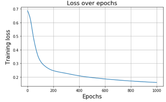
    optimizer.step() # Optimizer one step

When running 1000 epochs, you can easily generate all the familiar loss curves.

Want to see how probabilities change over time?

PyTorch allows for experimentation, exploration, breaking, and shaking things up.

Just for fun, if you want to check how the output layer probabilities evolve over multiple epochs, you can simply modify the previous code a bit,

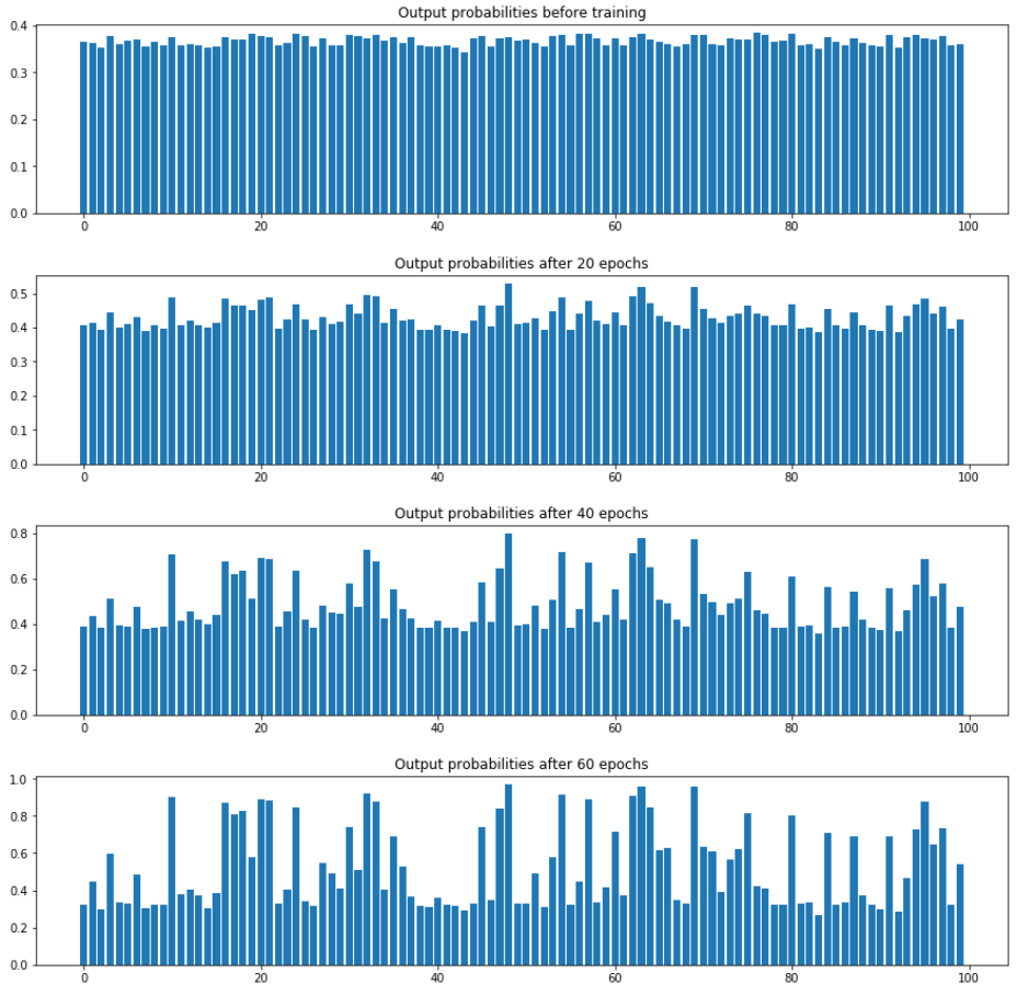
Clearly, the untrained network outputs are all close to 1, indicating no distinction between the positive and negative classes. As training continues, the probabilities separate from each other, gradually trying to match the distribution of the ground truth by adjusting the network’s weights.

PyTorch empowers you to experiment, explore, break, and shake things up.

Have other popular ideas? Try them out

PyTorch has been very popular since its early versions, especially among academic researchers and startups. The reason behind this is simple – it allows for trying out crazy ideas through simple code refactoring. Experimentation is at the core of new idea development in any scientific field, and deep learning is no exception.

Mixing with Two Activation Functions?

Just for (a bit) crazy, let’s say you want to mix it with two different activation functions – ReLU and Hyperbolic tangent (tanh). You want to split the tensor into two parallel parts, apply these activations to them separately, add the resulting tensors together, and then propagate it normally.

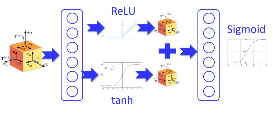
Does it seem complicated? Implement the desired code. Pass the input tensor (for example X) through the first hidden layer, then create two tensors X1 and X2 by letting the resulting tensor flow through separate activation functions. Just add the resulting tensors together and pass them through the second hidden layer.

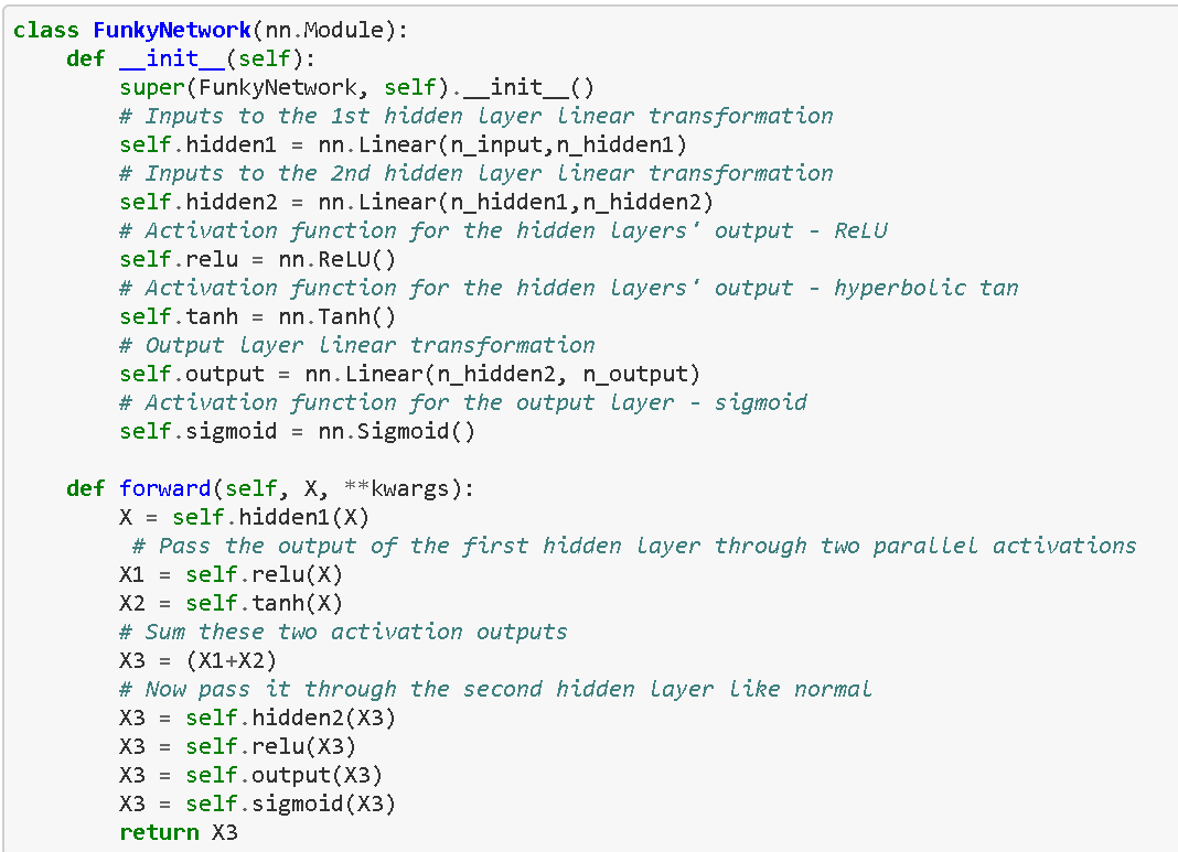
This kind of experimental work can be performed easily using PyTorch to change the architecture of the network.

Experimentation is at the core of new idea development in any scientific field, and deep learning is no exception.

Want to try your custom loss function?

You might want to try your custom loss function. Since high school, you have been using mean squared error. How about performing a quartic operation for regression problems?

Just define a function…

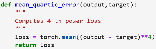
Then use it in the code (note that reg_model can be constructed by shutting off the S shaped activation in the output of the Network class).

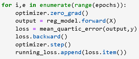
Now, does it feel like this?

Conclusion

All code for this demonstration can be found in the GitHub repository.

https://github.com/tirthajyoti/PyTorch_Machine_Learning

This article summarizes some key steps to quickly build neural networks for classification or regression tasks. It also demonstrates how to easily try clever ideas using this framework.

Heavy! The Yizhen Natural Language Processing – Academic WeChat group has been established

You can scan the QR code below to join the group for communication. Please avoid contacting the group owner or commercial agents. Thank you!

Recommended Reading:
Differences and Connections Between Fully Connected Graph Convolutional Networks (GCN) and Self-attention Mechanisms
Complete Guide for Beginners on Graph Convolutional Networks (GCN)
Paper Appreciation [ACL18] Based on Self-Attentive Constituency Parsing