Breakthrough LSTM! Multivariate Data Anomaly Detection with LSTM and KNN

Hello, I am Xiao Chu~

Today we are going to talk about a topic: using LSTM and KNN for multivariate data anomaly detection.

Related Principles

Multivariate Data Anomaly Detection is a very important task, especially in complex contexts such as high-dimensional data and time series data. Traditional anomaly detection methods (such as those based on statistical models or distance algorithms) often perform poorly in handling these complex data. LSTM (Long Short-Term Memory) and KNN (K-Nearest Neighbors) are two different algorithms, each adept at handling different types of data and problems, but they can complement each other in the task of multivariate data anomaly detection.

The Principle of LSTM (Long Short-Term Memory Network) in Multivariate Data Anomaly Detection

LSTM is a special structure based on Recurrent Neural Networks (RNN), adept at handling time series data, time-dependent data, and nonlinear dynamic systems. It solves the gradient vanishing problem in traditional RNNs through internal memory units and gating mechanisms, allowing it to capture long-term dependencies.

In the anomaly detection scenario, LSTM is used to learn the normal patterns of time series data. The specific process is as follows:

• Training Phase: The LSTM network is trained on a large amount of normal data to learn the complex relationships between the input at each moment and the historical states. In this way, LSTM can predict the expected output at the next moment.
• Detection Phase: During the detection process, for each new input data, LSTM can make predictions based on historical information. Then the predicted value is compared with the actual value, and if the prediction error exceeds a set threshold, the data at that moment is considered anomalous.

The working mechanism of LSTM includes the following three gates:

• Input Gate: Determines whether the current input should be saved to the memory unit.
• Forget Gate: Determines whether the previous information in the memory unit should be forgotten.
• Output Gate: Determines which information from the memory unit will affect the current output.

Formula Representation:

• State update formula for the memory unit:

Where, is the forget gate, is the input gate, is the candidate memory.

• Output formula:

Where, is the output gate, is the final output.

In anomaly detection, it can be determined whether there is an anomaly based on the prediction error of the LSTM network:

Where, is the actual observed value, is the predicted value of the LSTM network. If exceeds a certain threshold, it is considered that the data at that moment is anomalous.

The Principle of KNN (K-Nearest Neighbors Algorithm) in Multivariate Data Anomaly Detection

KNN is a distance-based non-parametric method suitable for static data, especially for non-sequential high-dimensional multivariate data. The basic idea is: for a given data point, by calculating its distance to other data points in the training set, the nearest neighbors are found, and based on the distance information of these neighbors, the point is judged to be anomalous or not.

In multivariate data anomaly detection, the working principle of KNN is as follows:

• Distance Calculation: For the data point to be detected, first calculate its distance to other data points. Common distance metrics include Euclidean distance, Manhattan distance, cosine distance, etc. For example, using Euclidean distance, given two data points and , their Euclidean distance is:

• Select Neighbors: Find the data points that are closest to and denote them as .
• Judge Anomaly: Determine whether is anomalous based on the distances of its neighbors. If the average distance or median distance to its neighbors is much greater than the average distance of most samples, it is considered an anomalous point.

KNN usually has two variants to implement anomaly detection:

• Global KNN: Calculate the K-nearest neighbor distances for all samples, then determine the anomaly score based on the size of the distances.
• Local Outlier Factor (LOF): Compared to Global KNN, the LOF method considers local density information and identifies anomalous points by comparing with the local density of its neighbors. The formula is as follows:

Where, is the local reachability density of point , defined as:

is the reachability distance of K nearest neighbors.

LSTM and KNN Combined for Multivariate Data Anomaly Detection

LSTM and KNN can be combined in the task of multivariate data anomaly detection to form a hybrid model that fully utilizes LSTM’s advantage in handling temporal dependencies and KNN’s ability to capture static distribution patterns.

Principle of LSTM-KNN Hybrid Model:

• LSTM for Feature Extraction: First, use LSTM to model the time series data and extract high-dimensional features at each moment. These features can be the hidden layer state or output layer state of LSTM. LSTM can capture the temporal dependencies of the data.
• KNN for Anomaly Detection: Use the features extracted from LSTM as input and apply KNN for anomaly detection on these features. KNN determines whether the current moment is anomalous based on the spatial distribution of the features.

Process Steps:

• Data Preprocessing: Standardize and normalize the time series data.
• LSTM Modeling: Train the LSTM model on normal data to extract features at each moment.
• KNN Detection: Use KNN on these features to determine whether the distance of each data point at that moment is too large compared to others, thereby judging anomalies.

Formula Summary:

• LSTM Part:

• KNN Part:

If is much larger than other points, it is judged as anomalous.

The advantage of this combined model is that it can handle complex dynamic relationships in time series while effectively addressing static anomalies in multivariate high-dimensional data, making it more widely applicable.

In summary:

• LSTM is suitable for handling time series data, capable of learning temporal dependencies and detecting anomalies through prediction errors.
• KNN is suitable for multivariate data space, discovering anomalous points through neighbor distances.
• LSTM-KNN Hybrid Model utilizes LSTM to extract time series features and combines KNN’s spatial distance judgment, which can better address the anomaly detection problem in complex multivariate data.

Complete Case Study

Multivariate data anomaly detection is a very important task in data analysis, especially in discovering anomalies in complex time series or high-dimensional data. This is widely used in industrial equipment fault detection, financial transaction fraud detection, and network traffic monitoring.

LSTM (Long Short-Term Memory Network) is a deep learning model specifically designed to handle time series, capable of capturing the temporal dependencies in data.KNN (K-Nearest Neighbors) is a distance-based non-parametric method suitable for anomaly detection in static multivariate data.

We use PyTorch to implement the LSTM model, extract time series features, and then use KNN for anomaly detection. For demonstration, we will generate a virtual multivariate time series dataset with artificial anomalies.

Steps:

1. Generate a virtual multivariate time series dataset and inject anomalies.
2. Use PyTorch to implement the LSTM model to train the data and extract features.
3. Use KNN to perform anomaly detection on the extracted features.
4. Visualize the results of anomaly detection.
5. Provide algorithm optimization points and parameter tuning processes.

1. Data Generation and Anomaly Injection

First, we need to generate a multivariate time series dataset and inject anomalies at certain time points.

import numpy as np
import pandas as pd
import matplotlib.pyplot as plt
from sklearn.preprocessing import MinMaxScaler
import torch
from torch.utils.data import DataLoader, TensorDataset

# Set random seed to ensure reproducibility
np.random.seed(42)

# Generate a virtual multivariate time series dataset (5 features, 1000 time points)
time_steps = 1000
features = 5
normal_data = np.random.randn(time_steps, features)

# Introduce a time trend
for i in range(features):
    normal_data[:, i] += np.sin(np.linspace(0, 20, time_steps)) * (i+1)

# Inject some anomalous data
anomalies = np.random.randn(50, features) * 5
anomaly_indices = np.random.choice(range(200, 800), 50, replace=False)
normal_data[anomaly_indices] = anomalies

# Generate DataFrame
df = pd.DataFrame(normal_data, columns=[f"feature_{i}" for i in range(features)])

# Normalize the data
scaler = MinMaxScaler()
scaled_data = scaler.fit_transform(df)

# Plot the first 100 time points of the dataset, including injected anomalies
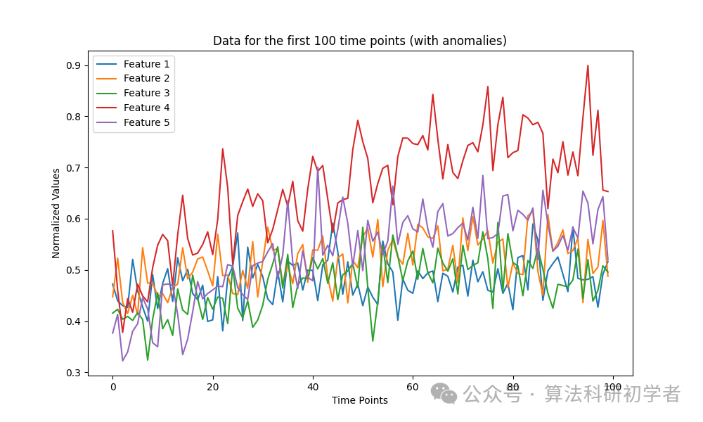
plt.figure(figsize=(10, 6))
for i in range(features):
    plt.plot(scaled_data[:100, i], label=f'Feature {i+1}')
plt.title("Data for the first 100 time points (with anomalies)")
plt.xlabel("Time Points")
plt.ylabel("Normalized Values")
plt.legend()
plt.show()

This graph shows the multiple feature values of the first 100 time points in the dataset, where anomalous data is randomly inserted and is significantly different from normal data.

2. Implementing LSTM Model with PyTorch

Next, we use PyTorch to implement the LSTM model to model the multivariate time series data and extract features.

import torch.nn as nn

# Define LSTM model
class LSTMModel(nn.Module):
    def __init__(self, input_size, hidden_size, output_size, num_layers):
        super(LSTMModel, self).__init__()
        self.hidden_size = hidden_size
        self.num_layers = num_layers
        
        # Define LSTM layer
        self.lstm = nn.LSTM(input_size, hidden_size, num_layers, batch_first=True)
        
        # Define fully connected layer
        self.fc = nn.Linear(hidden_size, output_size)

    def forward(self, x):
        h0 = torch.zeros(self.num_layers, x.size(0), self.hidden_size).to(device)
        c0 = torch.zeros(self.num_layers, x.size(0), self.hidden_size).to(device)

        out, _ = self.lstm(x, (h0, c0))  # LSTM output
        out = self.fc(out[:, -1, :])  # Only use the output of the last time step
        return out

# Convert data to PyTorch tensor
sequence_length = 10
X, y = [], []
for i in range(len(scaled_data) - sequence_length):
    X.append(scaled_data[i:i+sequence_length])
    y.append(scaled_data[i+sequence_length])

X = np.array(X)
y = np.array(y)

X_tensor = torch.tensor(X, dtype=torch.float32)
y_tensor = torch.tensor(y, dtype=torch.float32)

# Create DataLoader
batch_size = 32
dataset = TensorDataset(X_tensor, y_tensor)
train_loader = DataLoader(dataset, batch_size=batch_size, shuffle=True)

# Initialize model parameters
input_size = features
hidden_size = 64
output_size = features
num_layers = 2
device = torch.device('cuda' if torch.cuda.is_available() else 'cpu')

model = LSTMModel(input_size, hidden_size, output_size, num_layers).to(device)

# Define loss function and optimizer
criterion = nn.MSELoss()
optimizer = torch.optim.Adam(model.parameters(), lr=0.001)

# Train the model
num_epochs = 10
losses = []
for epoch in range(num_epochs):
    for batch_X, batch_y in train_loader:
        batch_X = batch_X.to(device)
        batch_y = batch_y.to(device)

        # Forward pass
        outputs = model(batch_X)
        loss = criterion(outputs, batch_y)
        
        # Backward pass and optimization
        optimizer.zero_grad()
        loss.backward()
        optimizer.step()
        
    losses.append(loss.item())
    print(f"Epoch [{epoch+1}/{num_epochs}], Loss: {loss.item():.4f}")

# Plot the loss changes during training
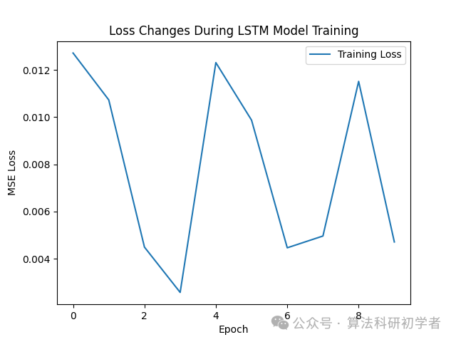
plt.plot(losses, label='Training Loss')
plt.title("Loss Changes During LSTM Model Training")

plt.xlabel("Epoch")
plt.ylabel("MSE Loss")
plt.legend()
plt.show()

This graph shows the loss changes during the training process of the LSTM model. It can be seen that as epochs increase, the loss gradually decreases, indicating that the model is learning the temporal dependency patterns of the data.

3. Using KNN for Anomaly Detection

Next, we extract the features at each time step from the LSTM model and use KNN for anomaly detection on these features.

from sklearn.neighbors import NearestNeighbors

# Use LSTM model to extract features
with torch.no_grad():
    lstm_features = model(X_tensor.to(device)).cpu().numpy()

# Use KNN for anomaly detection
knn = NearestNeighbors(n_neighbors=5)
knn.fit(lstm_features)

# Calculate the distance of each sample to its nearest neighbors
distances, indices = knn.kneighbors(lstm_features)

# Set anomaly threshold
anomaly_scores = distances.mean(axis=1)

# Plot anomaly scores
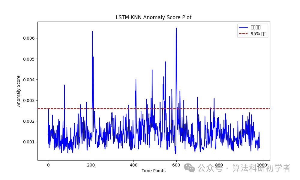
plt.figure(figsize=(10, 6))
plt.plot(anomaly_scores, label='Anomaly Score', color='b')
plt.axhline(y=np.percentile(anomaly_scores, 95), color='r', linestyle='--', label='95% Threshold')
plt.title("LSTM-KNN Anomaly Score Plot")
plt.xlabel("Time Points")
plt.ylabel("Anomaly Score")
plt.legend()
plt.show()

This graph illustrates the anomaly scores calculated by LSTM-KNN. The red dashed line indicates the 95% threshold for anomaly detection; time points exceeding this threshold are considered anomalous.

4. Visualizing Detection Results

Finally, we will compare the detected anomalies with the original data.

# Detect anomalies based on threshold
threshold = np.percentile(anomaly_scores, 95)
anomalies_detected = np.where(anomaly_scores > threshold)[0]

# Plot anomalies
plt.figure(figsize=(10, 6))
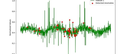
plt.plot(scaled_data[:, 0], label='Feature 1', color='g')
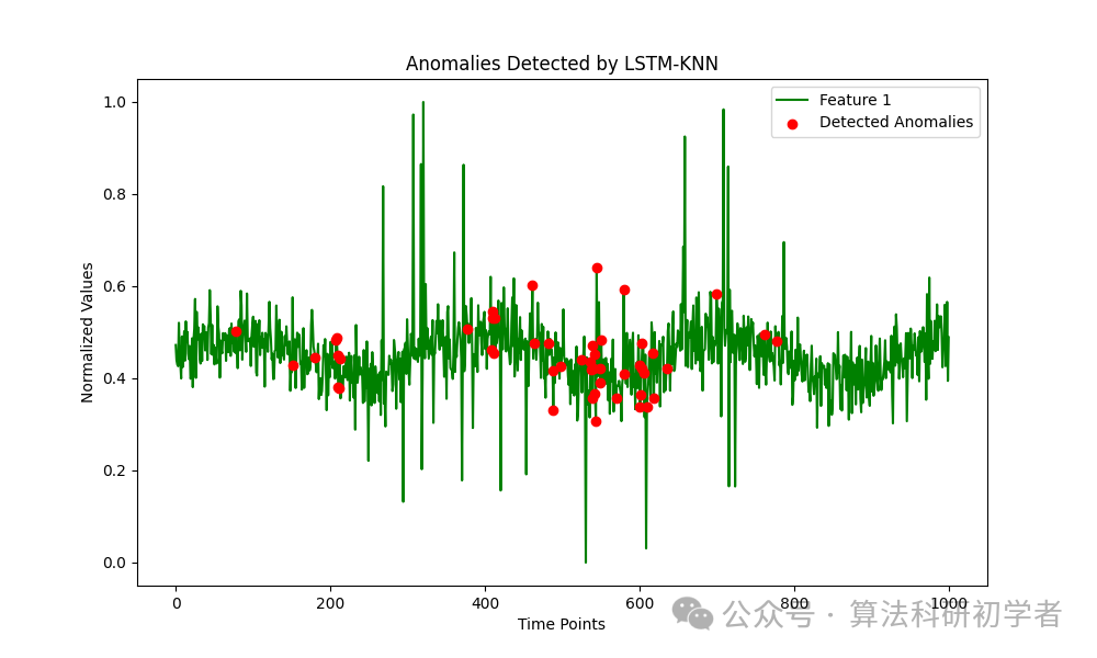
plt.scatter(anomalies_detected, scaled_data[anomalies_detected, 0], color='r', label='Detected Anomalies', zorder=5)
plt.title("Anomalies Detected by LSTM-KNN")
plt.xlabel("Time Points")
plt.ylabel("Normalized Values")
plt.legend()
plt.show()

This graph shows the anomalies detected by the LSTM-KNN model compared with the original data. The red points indicate the data points identified as anomalies, clearly showing their significant deviation from the normal data trend.

4. Algorithm Optimization Points and Parameter Tuning Process

1. Optimization Points

1. Design of LSTM Layers:

• Number of neurons in the hidden layer: More hidden units can usually capture more complexity of the data, but may also lead to overfitting.
• Number of LSTM layers: Increasing the number of LSTM layers can improve model performance, especially when handling more complex time series.

• Number of neighbors: A smaller will make the model very sensitive to local anomalies, while a larger will capture more global patterns. The value can be adjusted through cross-validation.
• Distance metric: Different distance metrics (such as Euclidean distance, Manhattan distance, etc.) can significantly impact detection results.

2. Parameter Tuning Process

1. Adjust LSTM Layer Count and Hidden Units:

• Experiment with different hidden unit counts (e.g., 32, 64, 128, etc.) and different layer counts (e.g., 1, 2, 3 layers) to select the configuration that performs best on the validation set.

• Try different values (e.g., 3, 5, 7) and calculate the model’s anomaly detection accuracy on the validation set.

• Use grid search or random search to automatically optimize the hyperparameters of LSTM and KNN.