Advancements in GAN: CGAN, DCGAN, WGAN, WGAN-GP, LSGAN, BEGAN
In the previous article, we introduced the principles of GAN (Introduction to Generative Adversarial Networks). The Generative Adversarial Network (GAN) mainly consists of two parts: the Generator and the Discriminator. The idea of the Generative model G is to package a random noise into a realistic sample, while the Discriminator model D needs to determine whether the input sample is real or a generated fake sample. Through adversarial training, both models improve together; the Discriminator D’s ability to distinguish samples continuously increases, and the Generator G’s ability to create fakes also improves. However, GANs face issues like training difficulties, the loss of the generator and discriminator not indicating the training process, and a lack of diversity in generated samples. Below, we introduce a series of improvements based on this.
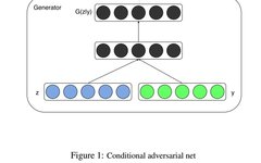
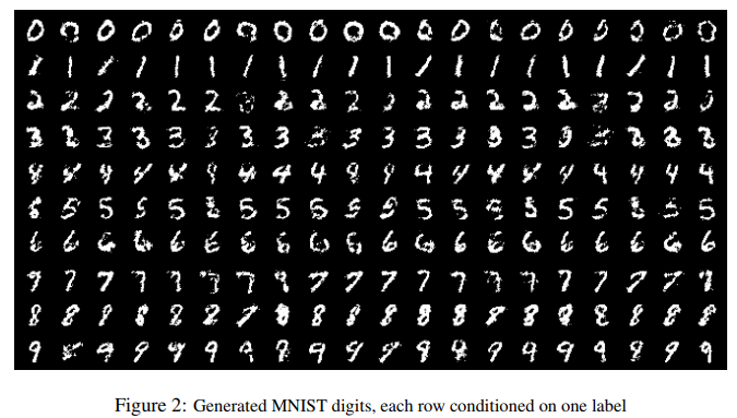
1. CGAN Conditional GAN Paper: Conditional Generative Adversarial Nets1. Principle The original GAN’s generation process could start training using random noise without needing a hypothesized data distribution. However, this free-form approach is less controllable for larger images. The CGAN method proposes a GAN with conditional constraints, adding conditions to the model through additional information to guide the data generation process. In this paper, the additional information y is fed into both the Discriminator and the Generator as part of the input layer, thus realizing a conditional GAN. This is based on the Mnist dataset, generating images of specified categories using category labels as conditional variables, transforming the purely unsupervised GAN into a supervised model.
2. Objective Function The objective function of conditional GAN is a two-player minimax game with conditional probabilities:

The network structure of CGAN:
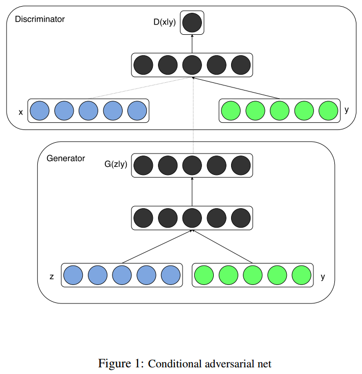
This paper focuses on the Mnist dataset, where the input to the generator is a 100-dimensional noise vector uniformly distributed, with category labels (one-hot encoding) as conditions to train the conditional GAN. The generator produces a single-channel image of 784 dimensions (28×28) through sigmoid activation, while the discriminator takes in 784-dimensional images and category labels (one-hot encoding) as input, outputting the probability that the sample comes from the training set.
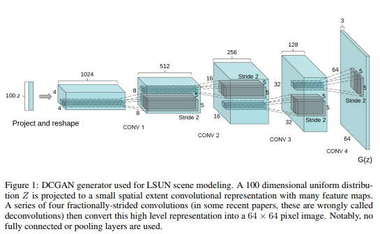
2. DCGAN Deep Convolutional GAN Paper: Unsupervised Representation Learning with Deep Convolutional Generative Adversarial Networks DCGAN replaces fully connected layers with convolutional layers and uses convolution with strides instead of upsampling, which better extracts image features. The Discriminator and Generator are symmetrically structured, greatly enhancing the stability of GAN training and the quality of generated results. The Discriminator employs leakyRELU instead of RELU to prevent gradient sparsity, while the Generator still uses RELU, but the output layer employs tanh. This paper uses the Adam optimizer to train GAN with a learning rate of 0.0002.The structure of the DCGAN generator is as follows, mapping 100-dimensional random noise input into an image through convolution:
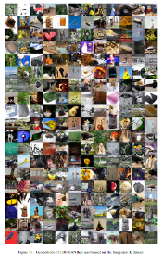
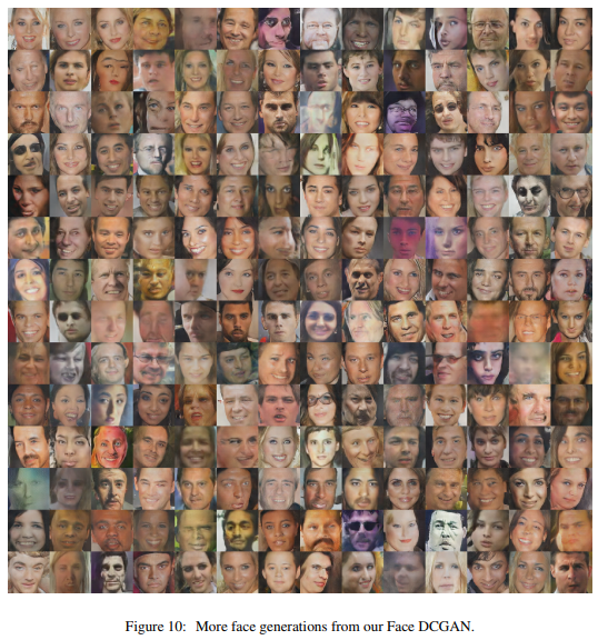
Some generated images are shown below:
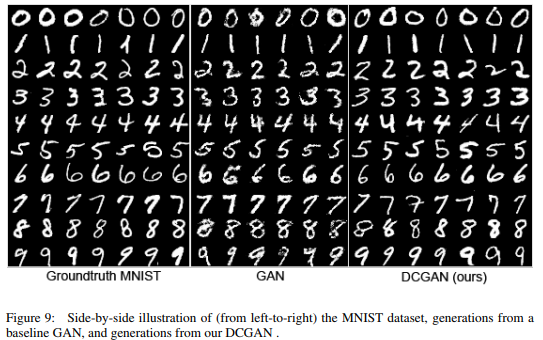
DCGAN does not fundamentally solve the instability of GAN training; care must still be taken to balance the training of the Generator and the Discriminator, often training one multiple times and the other once.
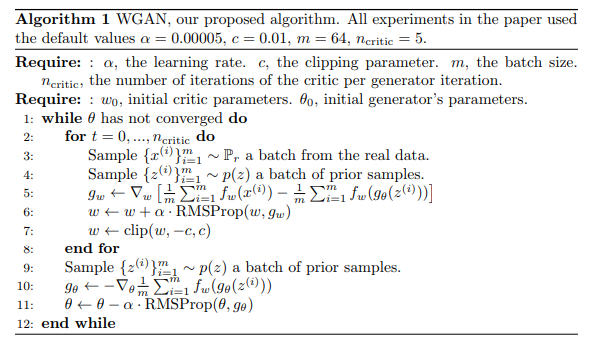
3. WGAN Paper: Wasserstein GAN WGAN mainly improves GAN from the perspective of loss function. This improvement can achieve good performance even in fully connected layers and theoretically explains the instability of GAN training, stating that the previous loss function (cross-entropy or JS divergence) is not suitable for measuring distances between distributions with non-overlapping parts. Instead, it uses the Wasserstein distance to measure the distance between the data distribution and the real data distribution, theoretically resolving the training instability issue, eliminating the need to carefully balance the training of the Generator and Discriminator. It also addresses the mode collapse problem (the generator tends to generate some confident but similar images and hesitates to try generating new images, resulting in a lack of diversity), making the Generator’s output more varied. Specific improvements include: 1) The last layer of the Discriminator removes the sigmoid; 2) The loss functions of the Generator and Discriminator do not include log; 3) After gradient updates, the weights are forced to be clipped within a certain range [-0.01, 0.01] to satisfy the Lipschitz continuity condition (which requires the gradient of the Discriminator function D(x) to not exceed a finite constant K in the sample space); 4) The paper suggests using other optimizers such as SGD or RMSprop instead of momentum-based optimization algorithms (momentum and Adam); 5) It proposes an evaluation metric to indicate the quality of GAN training during the process:
Problems with the Original Objective Function: The original GAN’s objective function is:

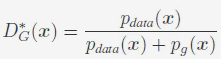
When the Generator is fixed, the optimal Discriminator is:
When the Discriminator is optimal, the optimization objective of the Generator is:
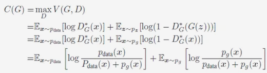
It can be expressed in the form of JS divergence:
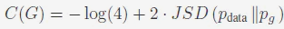
The aforementioned objective function related to JS divergence can lead to the problem of vanishing gradients. If the Discriminator is trained too well, the Generator cannot receive enough gradient for further optimization, and if the Discriminator is trained too weakly, its instructive role is not significant, which also prevents the Generator from learning effectively. Thus, controlling the training of the Discriminator becomes very difficult, which is the root of GAN training difficulties.
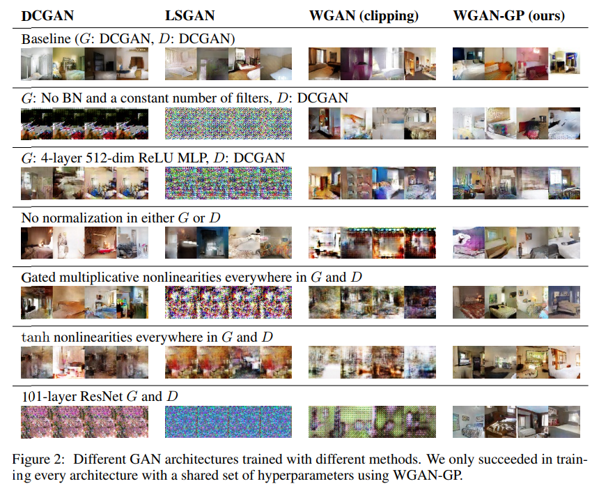
4. WGAN-GP Paper: Improved Training of Wasserstein GANs WGAN sometimes also faces issues like low sample quality and difficulty in convergence. WGAN-GP is an improved version of WGAN, mainly enhancing the Lipschitz continuity constraint. Previously, weight clipping was used to restrict weights to a certain range [-0.01, 0.01], but this approach is too simplistic, which can weaken the model’s modeling capability and cause gradient vanishing or explosion. WGAN-GP introduces Gradient Penalty,
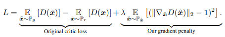
The design logic of the GP term is: a differentiable function satisfies the 1-Lipschitz condition only if its gradient norm does not exceed 1 at any point. Theoretically, the optimal Critic’s gradient norm should be close to 1 everywhere, which has little impact on the Lipschitz condition. Experimental results also show that two-sided penalty is slightly better than one-sided penalty. The detailed algorithm flow is as follows:
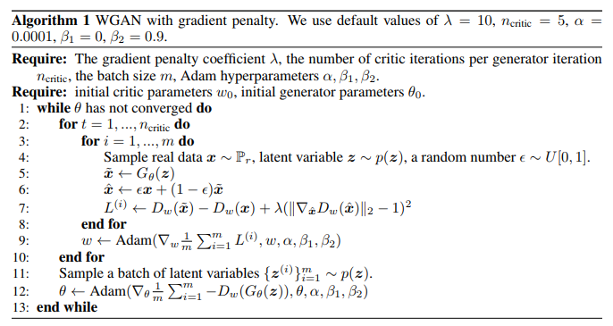
WGAN-GP outperforms WGAN in both training speed and the quality of generated samples. Since gradient penalties are applied to each sample in every batch (the dimension of the random number is (batchsize, 1)), batch normalization cannot be used in the Discriminator, but other normalization methods, such as Layer Normalization, Weight Normalization, and Instance Normalization, can be employed. The paper used Layer Normalization, and weight normalization also yields good results.
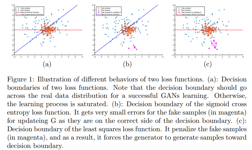
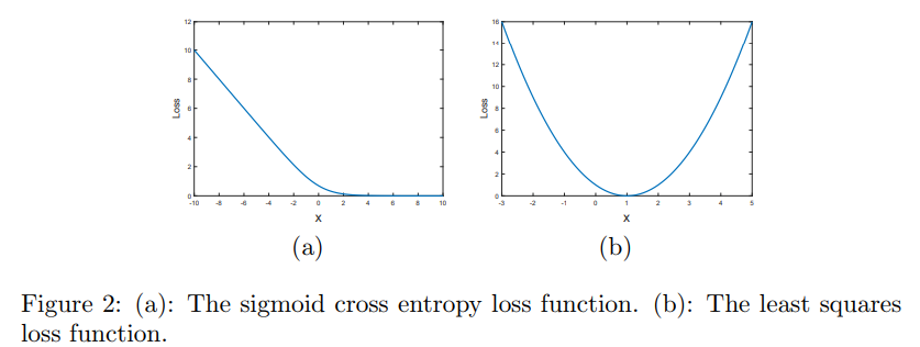
5. LSGAN Least Squares GAN Paper: Least Squares Generative Adversarial Networks LSGAN uses least squares loss function instead of the original GAN’s cross-entropy loss function, primarily addressing the issues of low image quality generated by the original GAN’s generator and the instability of the training process. The authors believe that using cross-entropy as a loss will prevent the generator from further optimizing those generated images recognized as real by the Discriminator, even if these generated images are still far from the decision boundary, meaning they are quite distant from the real data.This implies that the quality of the images generated by the Generator is not high.Why does the Generator stop optimizing the generated images?Because the Generator has already achieved the goal set for it—to confuse the Discriminator as much as possible, thus the cross-entropy loss is already quite low.In contrast, least squares loss is different; to minimize the least squares loss, the Generator must pull the generated images that are far from the decision boundary closer to it while still confusing the Discriminator.
The loss function is defined as follows:
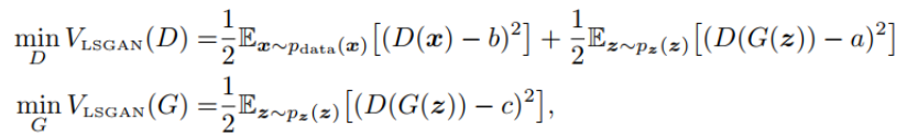
Sigmoid cross-entropy loss can easily reach saturation (saturation means the gradient is 0), while least squares loss only reaches saturation at one point, thus LSGAN makes GAN training more stable.
Some generated results are shown below:
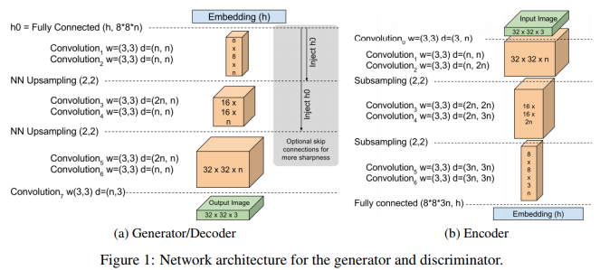
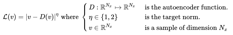
6. BEGAN (Boundary Equilibrium GAN) Boundary Equilibrium GAN Paper: BEGAN: Boundary Equilibrium Generative Adversarial Networks BEGAN is an improvement based on the equilibrium idea, which does not require training tricks, allowing for rapid and stable convergence using standard training steps. It maintains balance between the Discriminator and Generator during training. BEGAN employs an auto-encoder as the Discriminator, where the input is the image, and the output is the reconstructed image after encoding and decoding. It uses reconstruction error to measure whether a sample is generated or real, aiming to match the distribution of errors rather than the distribution of samples. If the distributions of errors are sufficiently close, then the distributions of real samples will also be sufficiently close, leading to high-quality generated images. BEGAN provides a hyperparameter that can balance between image diversity and generation quality, proposing a measure of convergence. The network structure is as follows:
The reconstruction error L(v) is:
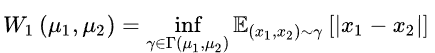
Let the mean of the reconstruction error distribution u1 of real samples be m1, and the mean of the reconstruction error distribution u2 of generated samples be m2, using EM distance to measure this distance:
Its lower bound is:

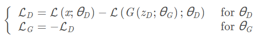
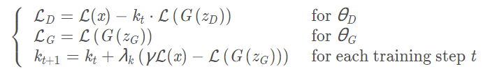
The loss functions corresponding to G and D in BEGAN are:
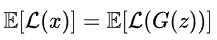
When the system reaches equilibrium, it should satisfy:
Introducing the hyperparameter diversity ratio for trade-off, when this value is small, D’s objective is to minimize the reconstruction error of real samples, while relatively less attention is paid to generated samples, leading to reduced diversity in the generated samples.
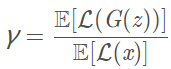
BEGAN’s objective is:
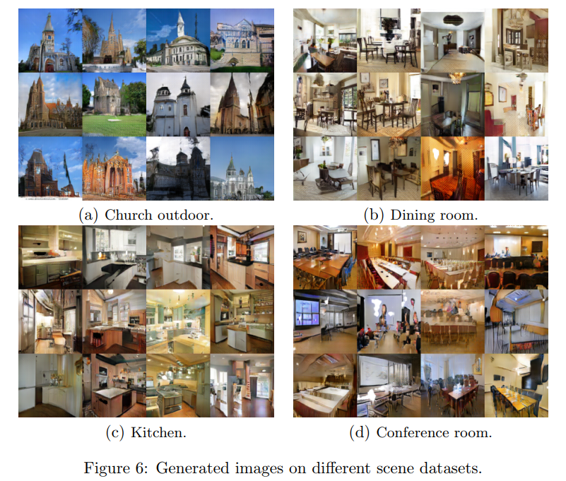
Some generated results are shown below:
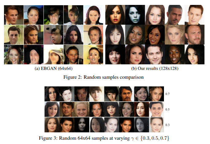
As hyperparameters change, the diversity and clarity of the generated results vary; smaller values yield clearer images but reduce diversity, while larger values decrease image quality but increase diversity.
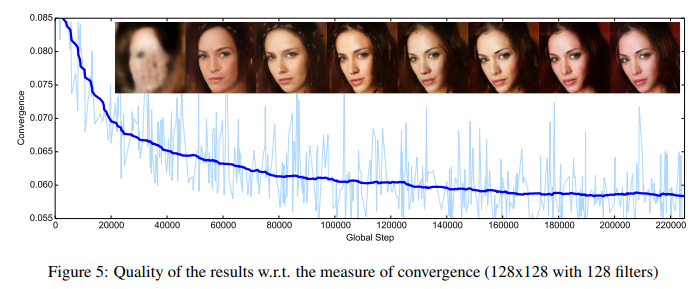
The above images show that as the model gradually converges, the quality of the generated images continuously improves.