A Comprehensive Overview of 11 Ingenious CNN Plugins

Introduction

This article reviews some of the more ingeniously designed and practical “plugins” used in CNN networks. The so-called “plugins” are modules that do not alter the main structure of the network and can be easily integrated into mainstream networks to enhance their feature extraction capabilities, achieving a plug-and-play functionality. Many similar reviews claim to offer plug-and-play solutions, but based on my experience and research, I have found that many plugins are impractical, non-generalizable, or even ineffective, which led to this article.

First, my understanding is: since they are “plugins,” they should be enhancements that are easy to implant and effectively usable, truly plug-and-play. The “plugins” listed in this article can be seen in many SOTA networks. These are conscientious “plugins” worth promoting, truly capable of plug-and-play functionality. In short, they are “plugins” that actually work. Many of these “plugins” have been developed to enhance CNN capabilities, such as translation, rotation, scale invariance, multi-scale feature extraction, receptive field enhancement, and spatial position awareness.

Nominees: STN, ASPP, Non-local, SE, CBAM, DCNv1&v2, CoordConv, Ghost, BlurPool, RFB, ASFF

STN

Source Paper: Spatial Transformer Networks

Paper Link: https://arxiv.org/pdf/1506.02025.pdf

Core Analysis:

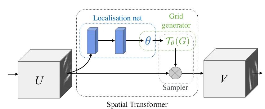
In tasks like OCR, you will often see its presence. For CNN networks, we hope they exhibit a certain invariance to object pose, location, etc. This means they should adapt to variations in pose and location in the test set. Invariance or equivariance can effectively enhance the model’s generalization ability. Although CNNs use sliding-window convolution operations, which provide some degree of translational invariance, many studies have found that downsampling can destroy this invariance. Thus, it can be concluded that the network’s invariance capability is very weak, let alone invariance to rotation, scale, and illumination. Generally, we use data augmentation to achieve network “invariance”.

This article proposes the STN module, which explicitly incorporates spatial transformations into the network, thereby enhancing the network’s invariance to rotation, translation, and scale. It can be understood as an “alignment” operation. The structure of STN is shown in the above image, where each STN module consists of a Localization net, a Grid generator, and a Sampler. The Localization net learns to obtain the parameters for spatial transformation, which are the six parameters in the equation above. The Grid generator is responsible for coordinate mapping, while the Sampler collects pixels using bilinear interpolation.

The significance of STN is that it can correct the original image into the ideal image desired by the network, and this process is performed in an unsupervised manner, meaning the transformation parameters are learned autonomously without the need for labeled information. This module is an independent module that can be inserted at any position in the CNN. It meets the criteria for this “plugin” review.

Core Code:

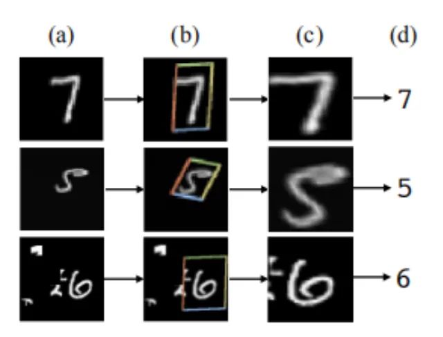
class SpatialTransformer(nn.Module):def __init__(self, spatial_dims):super(SpatialTransformer, self).__init__()self._h, self._w = spatial_dims self.fc1 = nn.Linear(32*4*4, 1024) # Set according to your network parametersself.fc2 = nn.Linear(1024, 6)def forward(self, x): batch_images = x # Save a copy of the original data x = x.view(-1, 32*4*4) # Learn the 6 parameters using FC structure x = self.fc1(x) x = self.fc2(x) x = x.view(-1, 2,3) # 2x3 # Generate sampling points using affine_grid affine_grid_points = F.affine_grid(x, torch.Size((x.size(0), self._in_ch, self._h, self._w))) # Apply sampling points to the original data rois = F.grid_sample(batch_images, affine_grid_points)return rois, affine_grid_points

ASPP

Full Name of Plugin: Atrous Spatial Pyramid Pooling

Source Paper: DeepLab: Semantic Image Segmentation with Deep Convolutional Nets, Atrous Conv

Paper Link: https://arxiv.org/pdf/1606.00915.pdf

Core Analysis:

This plugin is a spatial pyramid pooling module with dilated convolutions, primarily designed to enhance the network’s receptive field and introduce multi-scale information. We know that for semantic segmentation networks, they typically face high-resolution images, which require our networks to have a sufficient receptive field to cover the target objects. CNN networks generally rely on stacking convolutional layers and downsampling operations to acquire receptive fields. This module allows control of the receptive field size without altering the feature map size, which is beneficial for extracting multi-scale information. The rate controls the size of the receptive field; the larger the rate, the larger the receptive field.

ASPP mainly includes the following components: 1. A global average pooling layer to obtain image-level features, followed by a 1×1 convolution, which is bilinearly interpolated to the original size; 2. A 1×1 convolution layer and three 3×3 dilated convolutions; 3. The five different scale features are concatenated along the channel dimension and then passed through a 1×1 convolution for fusion output.

Core Code:

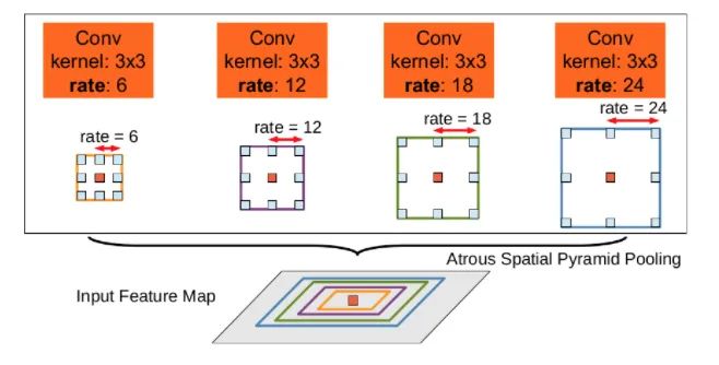
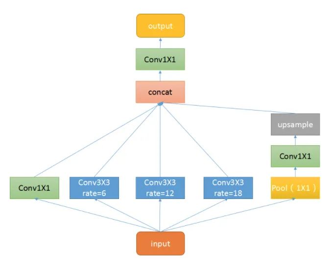
class ASPP(nn.Module):def __init__(self, in_channel=512, depth=256):super(ASPP,self).__init__()self.mean = nn.AdaptiveAvgPool2d((1, 1))self.conv = nn.Conv2d(in_channel, depth, 1, 1)self.atrous_block1 = nn.Conv2d(in_channel, depth, 1, 1) # Convolutions with different dilation ratesself.atrous_block6 = nn.Conv2d(in_channel, depth, 3, 1, padding=6, dilation=6)self.atrous_block12 = nn.Conv2d(in_channel, depth, 3, 1, padding=12, dilation=12)self.atrous_block18 = nn.Conv2d(in_channel, depth, 3, 1, padding=18, dilation=18)self.conv_1x1_output = nn.Conv2d(depth * 5, depth, 1, 1)def forward(self, x): size = x.shape[2:] # Pooling branch image_features = self.mean(x) image_features = self.conv(image_features) image_features = F.upsample(image_features, size=size, mode='bilinear') # Convolutions with different dilation rates atrous_block1 = self.atrous_block1(x) atrous_block6 = self.atrous_block6(x) atrous_block12 = self.atrous_block12(x) atrous_block18 = self.atrous_block18(x) # Merge features from all scales x = torch.cat([image_features, atrous_block1, atrous_block6, atrous_block12, atrous_block18], dim=1) # Use 1x1 convolution to fuse features for output x = self.conv_1x1_output(x)return net

Non-local

Source Paper: Non-local Neural Networks

Paper Link: https://arxiv.org/abs/1711.07971

Core Analysis:

Non-Local is an attention mechanism and is an easy-to-embed and integrate module. Local operations mainly target the receptive field; for example, in CNNs, the size of the receptive field is determined by the size of the convolution kernel, and we commonly use 3×3 convolution layers stacked together, which only consider local areas, thus performing local operations. In contrast, non-local operations can have a large receptive field, potentially covering a global area rather than just a local one. Capturing long-range dependencies, or how to establish connections between pixels that are a certain distance apart in an image, is a form of attention mechanism. The so-called attention mechanism utilizes the network to generate a saliency map, where attention corresponds to salient regions that the network should focus on.

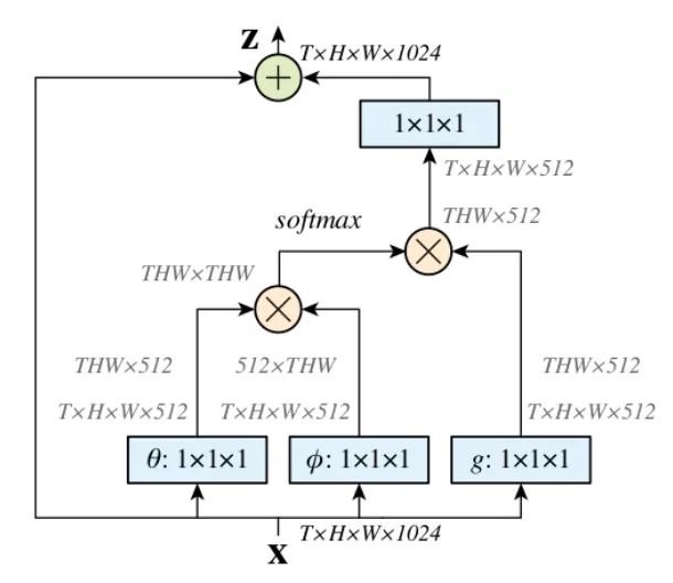
First, apply a 1×1 convolution to the input feature map to compress the channel number, obtaining, features.
Then, reshape the three features and perform matrix multiplication to obtain a covariance-like matrix. This step calculates the self-correlation in the features, i.e., the relationship of each pixel in each frame to every other pixel across all frames.
Next, apply a Softmax operation to the self-correlation features to obtain weights ranging from 0 to 1; these are the self-attention coefficients we need.
Finally, multiply the attention coefficients back onto the feature matrix g and add the residual from the original input feature map X for the output.

Let’s understand this with a simple example. Assume g is (we temporarily ignore the batch and channel dimensions):

g = torch.tensor([[1, 2], [3, 4]]).view(-1, 1).float()

Then,

theta = torch.tensor([2, 4, 6, 8]).view(-1, 1)

And,

phi = torch.tensor([7, 5, 3, 1]).view(1, -1)

Now, the matrix multiplication looks like this:

tensor([[14., 10.,  6.,  2.],[28., 20., 12.,  4.],[42., 30., 18.,  6.],[56., 40., 24.,  8.]])

After applying softmax(dim=-1), the result is as follows, where each row represents the importance of the elements in g; the larger values at the start of each row indicate that those elements should receive more “attention”. This can also be understood as the attention matrix representing the dependency level of each element in g with respect to others.

tensor([[9.8168e-01, 1.7980e-02, 3.2932e-04, 6.0317e-06],[9.9966e-01, 3.3535e-04, 1.1250e-07, 3.7739e-11],[9.9999e-01, 6.1442e-06, 3.7751e-11, 2.3195e-16],[1.0000e+00, 1.1254e-07, 1.2664e-14, 1.4252e-21]])

After applying the attention, the overall values converge towards 1:

tensor([[1.0187, 1.0003],[1.0000, 1.0000]])

Core Code:

class NonLocal(nn.Module):    def __init__(self, channel):super(NonLocalBlock, self).__init__()self.inter_channel = channel // 2self.conv_phi = nn.Conv2d(channel, self.inter_channel, 1, 1,0, False)self.conv_theta = nn.Conv2d(channel, self.inter_channel, 1, 1,0, False)self.conv_g = nn.Conv2d(channel, self.inter_channel, 1, 1, 0, False)self.softmax = nn.Softmax(dim=1)self.conv_mask = nn.Conv2d(self.inter_channel, channel, 1, 1, 0, False)def forward(self, x):# [N, C, H , W]        b, c, h, w = x.size()# Get phi features, dimension [N, C/2, H * W]        x_phi = self.conv_phi(x).view(b, c, -1)# Get theta features, dimension [N, H * W, C/2]        x_theta = self.conv_theta(x).view(b, c, -1).permute(0, 2, 1).contiguous()# Get g features, dimension [N, H * W, C/2]        x_g = self.conv_g(x).view(b, c, -1).permute(0, 2, 1).contiguous()# Matrix multiplication of phi and theta, [N, H * W, H * W]        mul_theta_phi = torch.matmul(x_theta, x_phi)# Apply softmax to bring values between 0 and 1        mul_theta_phi = self.softmax(mul_theta_phi)# Matrix multiplication with g features, [N, H * W, C/2]        mul_theta_phi_g = torch.matmul(mul_theta_phi, x_g)# [N, C/2, H, W]        mul_theta_phi_g = mul_theta_phi_g.permute(0, 2, 1).contiguous().view(b, self.inter_channel, h, w)# 1x1 convolution to expand channel numbers        mask = self.conv_mask(mul_theta_phi_g)out = mask + x # Residual connectionreturn out

Source Paper: Squeeze-and-Excitation Networks

Paper Link: https://arxiv.org/pdf/1709.01507.pdf

Core Analysis:

This paper is the champion work from the last ImageNet competition, and you can see it in many classic network structures, such as MobileNet v3. It is essentially a channel attention mechanism. Due to feature compression and the presence of FC layers, the captured channel attention features contain global information. This paper proposes a new structural unit called the “Squeeze-and-Excitation (SE)” module, which can adaptively adjust the feature response values of each channel and model the internal dependencies between channels. The steps are as follows:

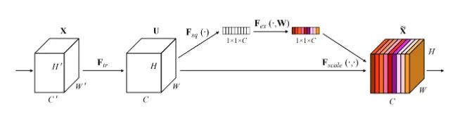
Squeeze: Compress features along the spatial dimension, reducing each 2D feature channel to a single value, which has a global receptive field.
Excitation: Each feature channel generates a weight representing the importance of that feature channel.
Reweight: The weights output from Excitation are treated as the importance of each feature channel and are applied multiplicatively to each channel.

Core Code:

class SE_Block(nn.Module):def __init__(self, ch_in, reduction=16):        super(SE_Block, self).__init__()        self.avg_pool = nn.AdaptiveAvgPool2d(1)  # Global adaptive pooling        self.fc = nn.Sequential(            nn.Linear(ch_in, ch_in // reduction, bias=False),            nn.ReLU(inplace=True),            nn.Linear(ch_in // reduction, ch_in, bias=False),            nn.Sigmoid()        )def forward(self, x):        b, c, _, _ = x.size()        y = self.avg_pool(x).view(b, c) # squeeze operation        y = self.fc(y).view(b, c, 1, 1) # FC to obtain channel attention weights, which contain global informationreturn x * y.expand_as(x) # Apply attention to each channel

CBAM

Source Paper: CBAM: Convolutional Block Attention Module

Paper Link: https://openaccess.thecvf.com/content_ECCV_2018/papers/Sanghyun_Woo_Convolutional_Block_Attention_ECCV_2018_paper.pdf

Core Analysis:

SENet focuses on obtaining attention weights at the channel level, which are then multiplied with the original feature maps. This article points out that this attention method only considers which layers have stronger feedback capabilities at the channel level but does not reflect attention at the spatial dimension. CBAM, as the highlight of this paper, applies attention simultaneously in both channel and spatial dimensions. Like the SE Module, CBAM can be embedded in most mainstream networks and can enhance the model’s feature extraction capabilities without significantly increasing computational and parameter loads.

Channel Attention: As shown in the figure, the input is a feature F of size H×W×C. We first apply global average pooling and max pooling separately to obtain two 1×1×C channel descriptors. Then, we send them through a two-layer neural network, with the first layer having C/r neurons and using ReLU as the activation function, and the second layer having C neurons. Note that this two-layer neural network is shared. Finally, the two obtained features are summed and passed through a Sigmoid activation function to obtain the weight coefficient Mc. The resulting weight coefficient is multiplied with the original feature F to obtain the scaled new feature. Pseudocode:

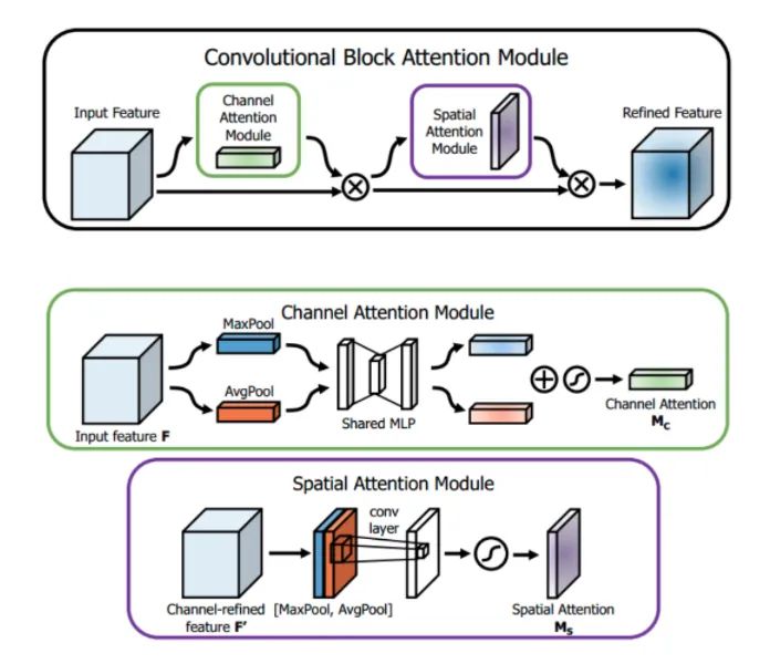
def forward(self, x):# Obtain global information using FC and perform matrix multiplication similar to Non-local    avg_out = self.fc2(self.relu1(self.fc1(self.avg_pool(x))))    max_out = self.fc2(self.relu1(self.fc1(self.max_pool(x))))    out = avg_out + max_outreturn self.sigmoid(out)

Spatial Attention: Similar to channel attention, given a feature F’ of size H×W×C, we first perform average pooling and max pooling along the channel dimension to obtain two H×W×1 channel descriptors, which are then concatenated along the channel dimension. After that, we pass this concatenated descriptor through a 7×7 convolution layer with a Sigmoid activation function to obtain the weight coefficient Ms. Finally, we multiply the weight coefficient with the feature F’ to obtain the scaled new feature. Pseudocode:

def forward(self, x):# Here we obtain global information using pooling    avg_out = torch.mean(x, dim=1, keepdim=True)    max_out, _ = torch.max(x, dim=1, keepdim=True)    x = torch.cat([avg_out, max_out], dim=1)    x = self.conv1(x)return self.sigmoid(x)

DCN v1&v2

Full Name of Plugin: Deformable Convolutional

Source Paper:

v1: [Deformable Convolutional Networks]

https://arxiv.org/pdf/1703.06211.pdf

v2: [Deformable ConvNets v2: More Deformable, Better Results]

https://arxiv.org/pdf/1811.11168.pdf

Core Analysis:

Deformable convolution can be seen as a combination of deformation and convolution, and thus can be used as a plugin. In many mainstream detection networks, deformable convolution is indeed a significant enhancement. There are numerous interpretations available online. Compared to traditional fixed-window convolutions, deformable convolutions can effectively adapt to geometric shapes because their “local receptive fields” are learnable and oriented towards the entire image. This paper also proposes deformable ROI pooling; both methods increase additional offsets for spatial sampling positions without requiring extra supervision, resulting in a self-supervised process.

As shown in the figure, a represents different convolutions, b represents deformable convolution, where the dark points indicate the actual sampling positions of the convolution kernel, which have some offsets from the “standard” positions. c and d represent special forms of deformable convolution, where c is the commonly seen dilated convolution, and d possesses the ability to learn rotation characteristics, also enhancing the receptive field.

Deformable convolution has two versions, V1 and V2, where V2 improves upon V1 by adding sampling weights alongside the sampling offsets. V2 suggests that 3×3 sampling points should also have varying importance, thus enhancing flexibility and fitting capabilities.

Core Code:

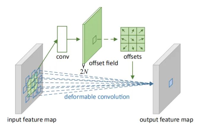
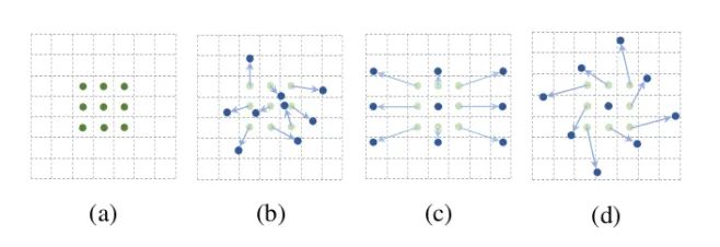
def forward(self, x):# Learn offsets, including x and y directions, note that each pixel in each channel has an x and y offset    offset = self.p_conv(x)if self.v2: # When V2, an additional weight coefficient is learned, passed through sigmoid to bring it between 0 and 1        m = torch.sigmoid(self.m_conv(x))# Use offsets to interpolate x, obtaining the offset x_offset    x_offset = self.interpolate(x,offset)if self.v2: # When V2, apply the weight coefficient to the feature map        m = m.contiguous().permute(0, 2, 3, 1)        m = m.unsqueeze(dim=1)        m = torch.cat([m for _ in range(x_offset.size(1))], dim=1)        x_offset *= m    out = self.conv(x_offset) # After applying the offset, perform standard convolutionreturn out

CoordConv

Source Paper: An intriguing failing of convolutional neural networks and the CoordConv solution

Paper Link: https://arxiv.org/pdf/1807.03247.pdf

Core Analysis:

In the Solo semantic segmentation algorithm and Yolov5, you can see its presence. This paper starts from several small experiments to explore the convolutional network’s ability to transform spatial representations into Cartesian coordinates. It shows that the network fails to convert spatial representations into coordinates in Cartesian space. As illustrated in the figure, when we input (i, j) coordinates into a network and require it to output a 64×64 image with a square or a pixel drawn at the coordinates, the network fails to achieve this on the test set, despite it being an extremely simple task for humans. The analysis reveals that convolution, being a local and weight-sharing filter applied to the input, does not know where each filter is located, making it unable to capture positional information. Therefore, we can assist the convolution by adding positional information to the input. This can be done simply by adding two channels: one for the i coordinate and another for the j coordinate. Specifically, as shown in the figure, we add two channels before feeding into the filters. This way, the network gains spatial positional awareness. Isn’t that fascinating? You can randomly use this plugin in classification, segmentation, detection, and other tasks.

In the first set of images above, traditional CNNs struggle to generate images based on coordinate values, performing well on the training set but poorly on the test set. After adding CoordConv in the second set of images, the task is easily accomplished, demonstrating that it enhances the CNN’s spatial perception capability.

Core Code:

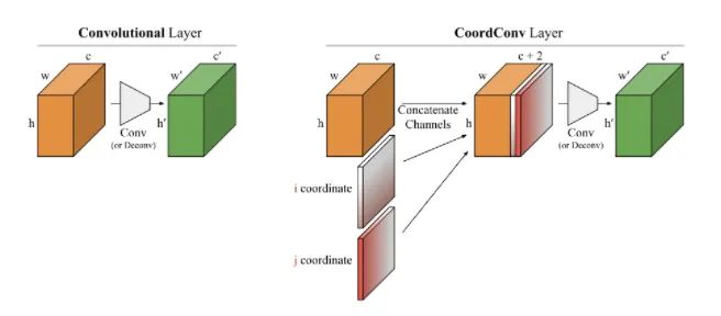
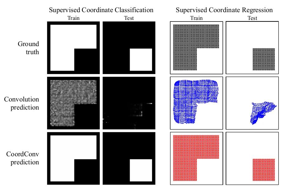
ins_feat = x # Current instance feature tensor# Generate linear values from -1 to 1x_range = torch.linspace(-1, 1, ins_feat.shape[-1], device=ins_feat.device)y_range = torch.linspace(-1, 1, ins_feat.shape[-2], device=ins_feat.device)y, x = torch.meshgrid(y_range, x_range) # Generate 2D coordinate gridy = y.expand([ins_feat.shape[0], 1, -1, -1]) # Expand to match ins_feat dimensionsx = x.expand([ins_feat.shape[0], 1, -1, -1])coord_feat = torch.cat([x, y], 1) # Position featuresins_feat = torch.cat([ins_feat, coord_feat], 1) # Concatenate as input for the next convolution

Ghost

Full Name of Plugin: Ghost module

Source Paper: GhostNet: More Features from Cheap Operations

Paper Link: https://arxiv.org/pdf/1911.11907.pdf

Core Analysis:

In the ImageNet classification task, GhostNet achieved a Top-1 accuracy of 75.7% under similar computational loads, outperforming MobileNetV3’s 75.2%. Its main innovation is the introduction of the Ghost module. In CNN models, feature maps often contain a lot of redundancy, which is indeed important and necessary. As illustrated in the figure, the feature maps marked with a “wrench” icon contain redundant features. So, can we reduce the number of convolution channels and then use some transformation to generate redundant feature maps? This is essentially the idea behind GhostNet.

This paper addresses the issue of redundancy in feature maps by proposing a structure that can generate a large number of feature maps with minimal computation (referred to as cheap operations). The cheap operations involve linear transformations, and the paper employs convolution operations to achieve this. The specific process is as follows:

Use fewer convolution operations than normal; for instance, instead of 64 convolution kernels, only use 32, halving the computational load.
Utilize depthwise separable convolutions to generate redundant features from the features obtained above.
Concatenate the features obtained from the above two steps for output, sending them to subsequent stages.

Core Code:

class GhostModule(nn.Module):    def __init__(self, inp, oup, kernel_size=1, ratio=2, dw_size=3, stride=1, relu=True):super(GhostModule, self).__init__()self.oup = oup        init_channels = math.ceil(oup / ratio)        new_channels = init_channels*(ratio-1)self.primary_conv = nn.Sequential(            nn.Conv2d(inp, init_channels, kernel_size, stride, kernel_size//2, bias=False),            nn.BatchNorm2d(init_channels),            nn.ReLU(inplace=True) if relu else nn.Sequential(), )# Cheap operations, note the use of grouped convolutions for channel separationself.cheap_operation = nn.Sequential(            nn.Conv2d(init_channels, new_channels, dw_size, 1, dw_size//2, groups=init_channels, bias=False),            nn.BatchNorm2d(new_channels),            nn.ReLU(inplace=True) if relu else nn.Sequential(),)def forward(self, x):        x1 = self.primary_conv(x)  # Main convolution operation        x2 = self.cheap_operation(x1) # Cheap transformation operationout = torch.cat([x1,x2], dim=1) # Concatenate bothreturn out[:,:self.oup,:,:]

BlurPool

Source Paper: Making Convolutional Networks Shift-Invariant Again

Paper Link: https://arxiv.org/abs/1904.11486

Core Analysis:

We all know that convolution operations based on sliding windows exhibit translational invariance, thus it is generally assumed that CNN networks possess translational invariance or equivariance. However, is this truly the case? In practice, CNNs are very sensitive; even a slight alteration of a pixel or a single-pixel shift can lead to significant changes in the CNN’s output, even resulting in incorrect predictions. This indicates a lack of robustness. Typically, we use data augmentation to achieve so-called invariance. This paper investigates the root cause of the degradation of invariance, which lies in downsampling. Whether it is Max Pooling, Average Pooling, or convolution operations with a stride greater than 1, any downsampling involving a stride greater than 1 results in the loss of translational invariance. The specific example shown in the figure below illustrates that even a shift of one pixel leads to significant discrepancies in the Max Pool output.

To maintain translational invariance, low-pass filtering can be applied before downsampling. Traditional max pooling can be decomposed into two parts: max with stride = 1 + downsampling. Therefore, the authors propose MaxBlurPool = max + blur + downsampling to replace the original max pooling. Experiments have shown that while this operation does not completely solve the loss of translational invariance, it significantly alleviates the issue.

Core Code:

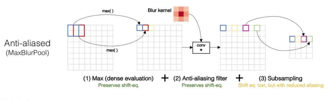
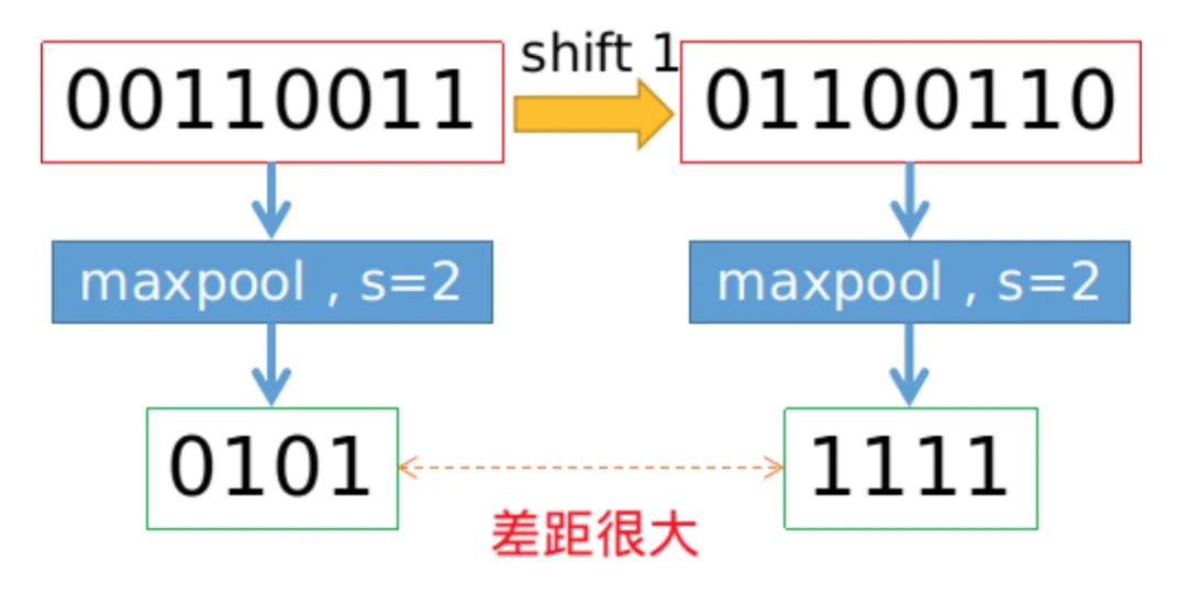
class BlurPool(nn.Module):def __init__(self, channels, pad_type='reflect', filt_size=4, stride=2, pad_off=0):super(BlurPool, self).__init__()self.filt_size = filt_sizeself.pad_off = pad_offself.pad_sizes = [int(1.*(filt_size-1)/2), int(np.ceil(1.*(filt_size-1)/2)), int(1.*(filt_size-1)/2), int(np.ceil(1.*(filt_size-1)/2))]self.pad_sizes = [pad_size+pad_off for pad_size in self.pad_sizes]self.stride = strideself.off = int((self.stride-1)/2.)self.channels = channels# Define a series of Gaussian kernelsif(self.filt_size==1):            a = np.array([1.,])        elif(self.filt_size==2):            a = np.array([1., 1.])        elif(self.filt_size==3):            a = np.array([1., 2., 1.])        elif(self.filt_size==4):                a = np.array([1., 3., 3., 1.])        elif(self.filt_size==5):                a = np.array([1., 4., 6., 4., 1.])        elif(self.filt_size==6):                a = np.array([1., 5., 10., 10., 5., 1.])        elif(self.filt_size==7):                a = np.array([1., 6., 15., 20., 15., 6., 1.])        filt = torch.Tensor(a[:,None]*a[None,:])        filt = filt/torch.sum(filt) # Normalization to ensure that the total information remains constant after blur# Non-grad parameters are stored using buffer self.register_buffer('filt', filt[None,None,:,:].repeat((self.channels,1,1,1)))self.pad = get_pad_layer(pad_type)(self.pad_sizes)def forward(self, inp):if(self.filt_size==1):if(self.pad_off==0):return inp[:,:,::self.stride,::self.stride]    else:return self.pad(inp)[:,:,::self.stride,::self.stride]else:# Use fixed parameters with conv2d+stride to implement blurpoolreturn F.conv2d(self.pad(inp), self.filt, stride=self.stride, groups=inp.shape[1])

RFB

Full Name of Plugin: Receptive Field Block

Source Paper: Receptive Field Block Net for Accurate and Fast Object Detection

Paper Link: https://arxiv.org/abs/1711.07767

Core Analysis:

This paper finds that the target area should be as close to the center of the receptive field as possible, which helps enhance the model’s robustness against small-scale spatial displacements. Inspired by the human visual RF structure, this paper proposes the Receptive Field Block (RFB), which strengthens the ability of CNN models to learn deep features, making detection models more accurate. RFB can be considered a universal module that can be embedded into most networks. The following figure illustrates its differences from inception, ASPP, and DCN, as it can be seen as a combination of inception and ASPP.

The specific implementation is shown in the figure below, which is similar to ASPP but uses different-sized convolution kernels as the precursor to dilated convolutions.

Core Code:

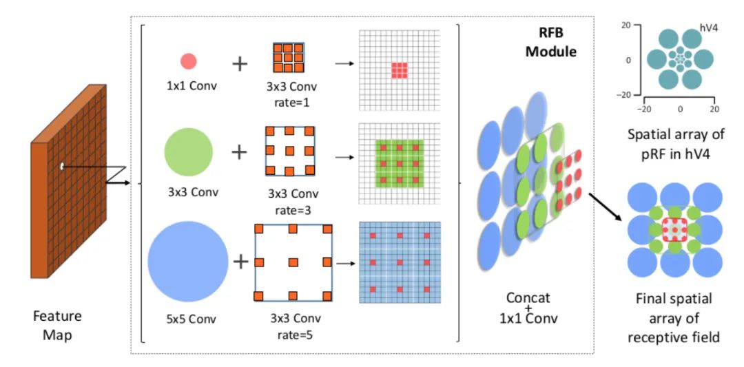
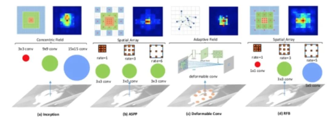
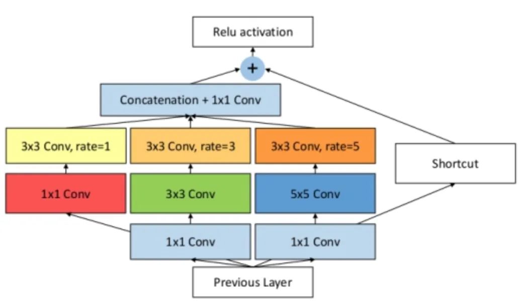
class RFB(nn.Module):    def __init__(self, in_planes, out_planes, stride=1, scale = 0.1, visual = 1):super(RFB, self).__init__()self.scale = scaleself.out_channels = out_planes        inter_planes = in_planes // 8# Branch 0: 1x1 convolution + 3x3 convolutionself.branch0 = nn.Sequential(conv_bn_relu(in_planes, 2*inter_planes, 1, stride),                conv_bn_relu(2*inter_planes, 2*inter_planes, 3, 1, visual, visual, False))# Branch 1: 1x1 convolution + 3x3 convolution + dilated convolutionself.branch1 = nn.Sequential(conv_bn_relu(in_planes, inter_planes, 1, 1),                conv_bn_relu(inter_planes, 2*inter_planes, (3,3), stride, (1,1)),                conv_bn_relu(2*inter_planes, 2*inter_planes, 3, 1, visual+1,visual+1,False))# Branch 2: 1x1 convolution + 3x3 convolution*3 instead of 5x5 convolution + dilated convolutionself.branch2 = nn.Sequential(conv_bn_relu(in_planes, inter_planes, 1, 1),                conv_bn_relu(inter_planes, (inter_planes//2)*3, 3, 1, 1),                conv_bn_relu((inter_planes//2)*3, 2*inter_planes, 3, stride, 1),                conv_bn_relu(2*inter_planes, 2*inter_planes, 3, 1, 2*visual+1, 2*visual+1,False))self.ConvLinear = conv_bn_relu(6*inter_planes, out_planes, 1, 1, False)self.shortcut = conv_bn_relu(in_planes, out_planes, 1, stride, relu=False)self.relu = nn.ReLU(inplace=False)    def forward(self,x):        x0 = self.branch0(x)        x1 = self.branch1(x)        x2 = self.branch2(x)# Scale fusionout = torch.cat((x0,x1,x2),1)# 1x1 convolutionout = self.ConvLinear(out)short = self.shortcut(x)out = out*self.scale + shortout = self.relu(out)return out

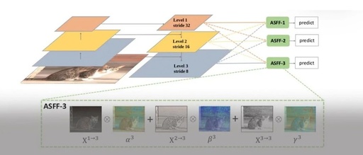
ASFF

Full Name of Plugin: Adaptively Spatial Feature Fusion

Source Paper: Adaptively Spatial Feature Fusion Learning Spatial Fusion for Single-Shot Object Detection

Paper Link: https://arxiv.org/abs/1911.09516v1

Core Analysis:

To make better use of high-level semantic features and low-level fine-grained features, many networks employ FPN to output multi-layer features; however, they often use concatenation or element-wise fusion methods. This paper argues that these methods do not fully utilize features of different scales, thus proposing an Adaptively Spatial Feature Fusion method. The feature maps output by FPN undergo the following two processes:

Feature Resizing: Different scales of feature maps cannot be fused element-wise, hence resizing is necessary. For upsampling: first apply a 1×1 convolution for channel compression, then use interpolation for upsampling the feature map. For downsampling by 1/2: use a 3×3 convolution with stride=2 for both channel compression and feature map reduction. For downsampling by 1/4: insert a max pooling operation with stride=2 before the 3×3 convolution with stride=2.

Adaptive Fusion: Features are fused adaptively, as shown in the formula below:

Where x n→l represents the feature vector at position (i, j) from the n feature map resized to the l scale. Alpha, Beta, and gamma are spatial attention weights processed through softmax, as follows:

Code Analysis:

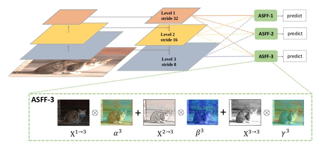
class ASFF(nn.Module):def __init__(self, level, rfb=False):super(ASFF, self).__init__()self.level = level# Input channels for the three feature layers, modify as neededself.dim = [512, 256, 256]self.inter_dim = self.dim[self.level]# The number of output channels for each layer must be consistentif level==0:self.stride_level_1 = conv_bn_relu(self.dim[1], self.inter_dim, 3, 2)self.stride_level_2 = conv_bn_relu(self.dim[2], self.inter_dim, 3, 2)self.expand = conv_bn_relu(self.inter_dim, 1024, 3, 1)        elif level==1:self.compress_level_0 = conv_bn_relu(self.dim[0], self.inter_dim, 1, 1)self.stride_level_2 = conv_bn_relu(self.dim[2], self.inter_dim, 3, 2)self.expand = conv_bn_relu(self.inter_dim, 512, 3, 1)        elif level==2:self.compress_level_0 = conv_bn_relu(self.dim[0], self.inter_dim, 1, 1)if self.dim[1] != self.dim[2]:self.compress_level_1 = conv_bn_relu(self.dim[1], self.inter_dim, 1, 1)self.expand = add_conv(self.inter_dim, 256, 3, 1)        compress_c = 8 if rfb else 16self.weight_level_0 = conv_bn_relu(self.inter_dim, compress_c, 1, 1)self.weight_level_1 = conv_bn_relu(self.inter_dim, compress_c, 1, 1)self.weight_level_2 = conv_bn_relu(self.inter_dim, compress_c, 1, 1)self.weight_levels = nn.Conv2d(compress_c*3, 3, 1, 1, 0)# Scale sizes level_0 < level_1 < level_2def forward(self, x_level_0, x_level_1, x_level_2):# Feature Resizing processif self.level==0:            level_0_resized = x_level_0            level_1_resized = self.stride_level_1(x_level_1)            level_2_downsampled_inter =F.max_pool2d(x_level_2, 3, stride=2, padding=1)            level_2_resized = self.stride_level_2(level_2_downsampled_inter)        elif self.level==1:            level_0_compressed = self.compress_level_0(x_level_0)            level_0_resized =F.interpolate(level_0_compressed, 2, mode='nearest')            level_1_resized =x_level_1            level_2_resized =self.stride_level_2(x_level_2)        elif self.level==2:            level_0_compressed = self.compress_level_0(x_level_0)            level_0_resized =F.interpolate(level_0_compressed, 4, mode='nearest')if self.dim[1] != self.dim[2]:                level_1_compressed = self.compress_level_1(x_level_1)                level_1_resized = F.interpolate(level_1_compressed, 2, mode='nearest')else:                level_1_resized =F.interpolate(x_level_1, 2, mode='nearest')            level_2_resized =x_level_2# Fusion weights are also learned by the network        level_0_weight_v = self.weight_level_0(level_0_resized)        level_1_weight_v = self.weight_level_1(level_1_resized)        level_2_weight_v = self.weight_level_2(level_2_resized)        levels_weight_v = torch.cat((level_0_weight_v, level_1_weight_v,                                     level_2_weight_v),1)        levels_weight = self.weight_levels(levels_weight_v)        levels_weight = F.softmax(levels_weight, dim=1)   # alpha generation# Adaptive fusion        fused_out_reduced = level_0_resized * levels_weight[:,0:1,:,:]+\                            level_1_resized * levels_weight[:,1:2,:,:]+\\                            level_2_resized * levels_weight[:,2:,:,:]        out = self.expand(fused_out_reduced)return out

Conclusion

This article has reviewed several ingeniously designed and practical CNN plugins from recent years, hoping that everyone can apply them effectively in their own projects.

Major Event

The GTIC 2021 Embedded AI Innovation Summit is officially launched! Four major sections showcase technological breakthroughs in embedded AI, the overall ecology, and application cases and practical explorations in the home AIoT, mobile robotics, and industrial manufacturing sectors. The audience registration channel is now fully open, and everyone can click on the poster to scan the code for registration. We will review and confirm as soon as possible.

Leave a Comment Cancel reply