Source:DeepHub IMBA
Complete code and detailed explanation for end-to-end time series forecasting using LSTM.
First, let’s understand two topics:
-
What is Time Series Analysis?
-
Time Series Analysis: A time series represents a series of data points indexed in time order. It can be in seconds, minutes, hours, days, weeks, months, or years. Future data will depend on its previous values.
In real-world cases, we mainly have two types of time series analysis:
For univariate time series data, we will use a single column for forecasting.
As we can see, there is only one column, so the upcoming future values will only depend on its previous values.
However, in the case of multivariate time series data, there will be different types of feature values, and the target data will depend on these features.
As seen in the image, there will be multiple columns in multivariate data to predict the target value. (In the above image, “count” is the target value)
In the above data, the count depends not only on its previous values but also on other features. Therefore, to predict the upcoming count value, we must consider all columns, including the target column, to make predictions.
One thing to remember when performing multivariate time series analysis is that we need to use multiple features to predict the current target. Let’s understand this through an example:
During training, if we use 5 columns [feature1, feature2, feature3, feature4, target] to train the model, we need to provide 4 columns [feature1, feature2, feature3, feature4] for the upcoming prediction day.
This article does not intend to discuss LSTM in detail. So here’s a brief description; if you are not very familiar with LSTM, you can refer to our previously published articles.
LSTM is basically a type of recurrent neural network that can handle long-term dependencies.
Imagine you are watching a movie. So when something happens in the movie, you already know what happened before and can understand that new situations arise because of past events. RNNs work in the same way; they remember past information and use it to process current inputs. The problem with RNNs is that they cannot remember long-term dependencies due to vanishing gradients. Thus, LSTM was designed to avoid the long-term dependency problem.
Now that we have discussed time series forecasting and the theoretical part of LSTM, let’s start coding.
First, let’s import the libraries needed for prediction:
import numpy as np
import pandas as pd
from matplotlib import pyplot as plt
from tensorflow.keras.models import Sequential
from tensorflow.keras.layers import LSTM
from tensorflow.keras.layers import Dense, Dropout
from sklearn.preprocessing import MinMaxScaler
from keras.wrappers.scikit_learn import KerasRegressor
from sklearn.model_selection import GridSearchCV
Load the data and check the output:
df=pd.read_csv("train.csv",parse_dates=["Date"],index_col=[0])
df.head()
Now let’s take some time to look at the data: The csv file contains stock data from Google from 2001-01-25 to 2021-09-29, with data recorded on a daily frequency.
[If you wish, you can convert the frequency to “B” [business days] or “D” since we will not use the dates; I just keep it as is.]
Here we are trying to predict the future values of the “Open” column, hence “Open” is the target column here.
Let’s look at the shape of the data:
df.shape(5203,5)
Now let’s perform a train-test split. Here we cannot shuffle the data because it must be ordered in time series.
test_split=round(len(df)*0.20)
df_for_training=df[:-1041]
df_for_testing=df[-1041:]
print(df_for_training.shape)
print(df_for_testing.shape)
(4162, 5)
(1041, 5)
It can be noted that the data range is very large and they are not scaled within the same range, so to avoid prediction errors, let’s first scale the data using MinMaxScaler. (StandardScaler can also be used)
scaler = MinMaxScaler(feature_range=(0,1))
df_for_training_scaled = scaler.fit_transform(df_for_training)
df_for_testing_scaled=scaler.transform(df_for_testing)
df_for_training_scaled
Split the data into X and Y, this is the most important part, read each step carefully.
def createXY(dataset,n_past):
 dataX = []
 dataY = []
 for i in range(n_past, len(dataset)):
 dataX.append(dataset[i - n_past:i, 0:dataset.shape[1]])
 dataY.append(dataset[i,0])
 return np.array(dataX),np.array(dataY)
trainX,trainY=createXY(df_for_training_scaled,30)
testX,testY=createXY(df_for_testing_scaled,30)
Let’s see what the above code does:
N_past is the number of steps we will look back at to predict the next target value.
Here we use 30, meaning we will use the past 30 values (including all features) to predict the 31st target value.
Thus, in trainX we will have all feature values, while in trainY we only have the target value.
Let’s break down each part of the for loop:
For training, dataset = df_for_training_scaled, n_past=30
data_X.addend (df_for_training_scaled[i - n_past:i, 0:df_for_training.shape[1]])
The range starts from n_past which is 30, so the first data range will be -[30 – 30,30,0:5] equivalent to [0:30,0:5]
So the first array in dataX will be df_for_training_scaled[0:30,0:5].
Now, dataY.append(df_for_training_scaled[i,0])
i = 30, so it will only take the open value from the 30th row (because in prediction, we only need the open column, so the column range is only 0, which indicates the open column).
The first value stored in the dataY list will be df_for_training_scaled[30,0].
So the first 30 rows containing 5 columns are stored in trainX, and only the open value of the 31st row is stored in trainY. Then we convert the dataX and dataY lists into arrays, which are trained in LSTM in array format.
Let’s take a look at the shapes.
print("trainX Shape-- ",trainX.shape)
print("trainY Shape-- ",trainY.shape)
(4132, 30, 5)
(4132,)
print("testX Shape-- ",testX.shape)
print("testY Shape-- ",testY.shape)
(1011, 30, 5)
(1011,)
4132 is the total number of arrays available in trainX, each array has 30 rows and 5 columns, and in each array of trainY, we have the next target value to train the model.
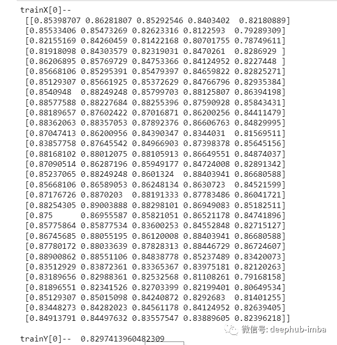
Let’s take a look at one of the arrays containing (30,5) data from trainX and the trainY value from the trainX array:
print("trainX[0]-- \n",trainX[0])
print("trainY[0]-- ",trainY[0])
If you look at the trainX[1] value, you will find it has the same data as in trainX[0] (except for the first column), because we will look at the first 30 to predict the 31st column, after the first prediction it will automatically move to the 2nd column and take the next 30 values to predict the next target value.
Let’s explain everything in a simple format:
trainX — — →trainY
[0 : 30,0:5] → [30,0]
[1:31, 0:5] → [31,0]
[2:32,0:5] →[32,0]
In this way, each data will be stored in trainX and trainY.
Now let’s train the model. I will use GridSearchCV for some hyperparameter tuning to find the base model.
def build_model(optimizer):
 grid_model = Sequential()
 grid_model.add(LSTM(50,return_sequences=True,input_shape=(30,5)))
 grid_model.add(LSTM(50))
 grid_model.add(Dropout(0.2))
 grid_model.add(Dense(1))
 grid_model.compile(loss = 'mse',optimizer = optimizer)
 return grid_model
grid_model = KerasRegressor(build_fn=build_model,verbose=1,validation_data=(testX,testY))
parameters = {'batch_size' : [16,20],            'epochs' : [8,10],            'optimizer' : ['adam','Adadelta'] }
grid_search = GridSearchCV(estimator = grid_model,                          param_grid = parameters,                          cv = 2)
If you want to do more hyperparameter tuning for your model, you can add more layers. But if the dataset is very large, it is recommended to increase the epochs and units in the LSTM model.
In the first LSTM layer, the input shape is (30,5). It comes from the shape of trainX.
(trainX.shape[1],trainX.shape[2]) → (30,5)
Now let’s fit the model to trainX and trainY data.
grid_search = grid_search.fit(trainX,trainY)
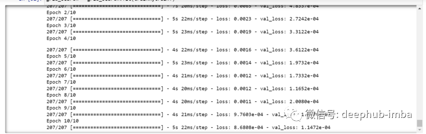
Since hyperparameter search is performed, this will take some time to run.
You can see the loss decreasing like this:
Now let’s check the best parameters of the model.
grid_search.best_params_
{'batch_size': 20, 'epochs': 10, 'optimizer': 'adam'}
Save the best model in the my_model variable.
my_model=grid_search.best_estimator_.model
Now we can test the model with the test dataset.
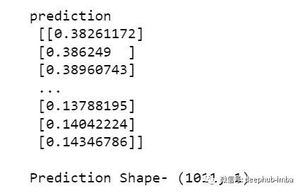
prediction=my_model.predict(testX)
print("prediction\n", prediction)
print("\nPrediction Shape-",prediction.shape)
The lengths of testY and prediction are the same. Now we can compare testY with the predictions.
However, we scaled the data at the beginning, so first we must perform some inverse scaling process.
scaler.inverse_transform(prediction)
There was an error because we have 5 columns in each row when scaling the data, but now we only have 1 column which is the target column.
So we must change the shape to use inverse_transform:
prediction_copies_array = np.repeat(prediction,5, axis=-1)
The 5 column values are similar; it just copies the single predicted column 4 times. So now we have 5 columns with the same values.
prediction_copies_array.shape(1011,5)
Now we can use the inverse_transform function.
pred=scaler.inverse_transform(np.reshape(prediction_copies_array,(len(prediction),5)))[:,0]
But the first column after inverse transformation is what we need, so we used → [:,0] at the end.
Now let’s compare this pred value with testY, but testY is also scaled and needs to be inverse transformed using the same code as above.
original_copies_array = np.repeat(testY,5, axis=-1)
original=scaler.inverse_transform(np.reshape(original_copies_array,(len(testY),5)))[:,0]
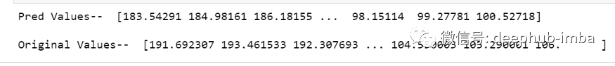
Now let’s take a look at the predicted values and the original values:
print("Pred Values-- " ,pred)
print("\nOriginal Values-- " ,original)
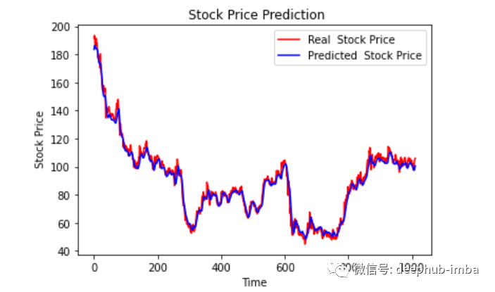
Finally, let’s plot a graph to compare our pred and original data.
plt.plot(original, color = 'red', label = 'Real Stock Price')
plt.plot(pred, color = 'blue', label = 'Predicted Stock Price')
plt.title('Stock Price Prediction')
plt.xlabel('Time')
plt.ylabel('Google Stock Price')
plt.legend()
plt.show()
It looks good so far; we have trained the model and checked it with the test values. Now let’s predict some future values.
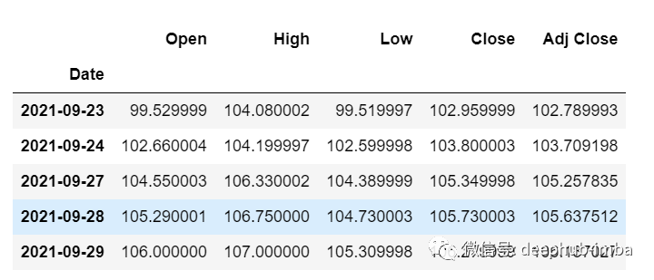
Get the last 30 values from the main df dataset that we loaded at the beginning [Why 30? Because this is the number of past values we want to predict the 31st value]
df_30_days_past=df.iloc[-30:,:]
df_30_days_past.tail()
We can see all columns including the target column (“Open”). Now let’s predict the next 30 values.
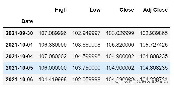
In multivariate time series forecasting, we need to predict a single column using different features, so when making predictions we need to use feature values (excluding the target column).
Here we need the upcoming 30 values of the “High”, “Low”, “Close”, and “Adj Close” columns to predict the “Open” column.
df_30_days_future=pd.read_csv("test.csv",parse_dates=["Date"],index_col=[0])
df_30_days_future
Before using the model for prediction, we need to do the following operations after removing the “Open” column:
Scale the data by adding an “Open” column with all values as “0” before scaling it.
After scaling, replace the “Open” column values in the future data with “nan”.
Now concatenate the 30 days old values and 30 days new values (where the last 30 “Open” values are nan)
df_30_days_future["Open"]=0
df_30_days_future=df_30_days_future[["Open","High","Low","Close","Adj Close"]]
old_scaled_array=scaler.transform(df_30_days_past)
new_scaled_array=scaler.transform(df_30_days_future)
new_scaled_df=pd.DataFrame(new_scaled_array)
new_scaled_df.iloc[:,0]=np.nan
full_df=pd.concat([pd.DataFrame(old_scaled_array),new_scaled_df]).reset_index().drop(["index"],axis=1)
The full_df shape is (60,5), with the first column having 30 nan values.
To make predictions, we must again use a for loop, as we did when splitting the trainX and trainY data. But this time we only have X without Y values.
full_df_scaled_array=full_df.values
all_data=[]
time_step=30
for i in range(time_step,len(full_df_scaled_array)):
 data_x=[]
 data_x.append(    full_df_scaled_array[i-time_step :i , 0:full_df_scaled_array.shape[1]])
 data_x=np.array(data_x)
 prediction=my_model.predict(data_x)
 all_data.append(prediction)
 full_df.iloc[i,0]=prediction
For the first prediction, it will check the previous 30 values when the for loop runs for the first time and predict the 31st “Open” data.
When the second for loop tries to run, it will skip the first row and attempt to get the next 30 values [1:31]. Here an error will occur because the last row of the Open column is “nan”, so it needs to replace “nan” with the prediction each time.
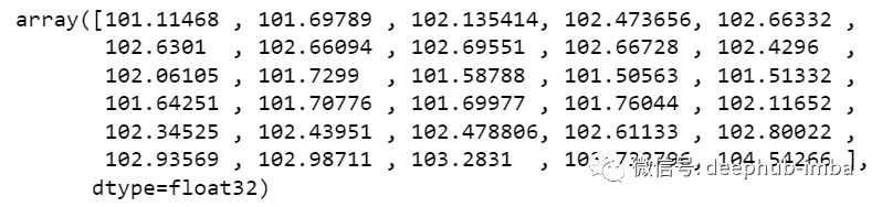
Finally, we also need to perform inverse transformation on the predictions:
new_array=np.array(all_data)
new_array=new_array.reshape(-1,1)
prediction_copies_array = np.repeat(new_array,5, axis=-1)
y_pred_future_30_days = scaler.inverse_transform(np.reshape(prediction_copies_array,(len(new_array),5)))[:,0]
print(y_pred_future_30_days)
This completes a full process.
If you want to see the complete code, you can check it here:
https://github.com/sksujan58/Multivariate-time-series-forecasting-using-LSTM