

1. Supervised Learning:
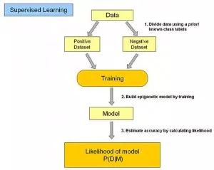
In supervised learning, the input data is called “training data,” and each set of training data has a clear label or result, such as “spam” or “not spam” in a spam detection system, or “1”, “2”, “3”, “4” in handwritten digit recognition. When building a predictive model, supervised learning establishes a learning process that compares the predicted results with the actual results of the “training data,” continuously adjusting the predictive model until the model’s predictions reach a desired accuracy.Common applications of supervised learning include classification problems and regression problems.Common algorithms include Logistic Regression and Back Propagation Neural Network.
2. Unsupervised Learning:
In unsupervised learning, the data is not specifically labeled, and the learning model is intended to infer some intrinsic structure of the data.Common application scenarios include learning association rules and clustering.Common algorithms include Apriori and k-Means.
3. Semi-Supervised Learning:
In this learning method, part of the input data is labeled, while some is not. This learning model can be used for prediction, but the model first needs to learn the intrinsic structure of the data to reasonably organize the data for prediction. Application scenarios include classification and regression, with algorithms including some extensions of common supervised learning algorithms that first attempt to model unlabeled data and then predict the labeled data based on that. For example, Graph Inference or Laplacian SVM.
4. Reinforcement Learning:
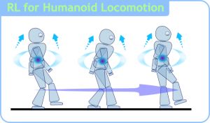
In this learning model, the input data serves as feedback to the model. Unlike supervised models where the input data is merely a way to check the correctness of the model, in reinforcement learning, the input data directly feeds back to the model, which must immediately adjust accordingly. Common application scenarios include dynamic systems and robot control.Common algorithms include Q-Learning and Temporal Difference Learning.
In the context of enterprise data applications, the most commonly used models are likely supervised learning and unsupervised learning. In fields like image recognition, where there is a large amount of unlabeled data and a small amount of labeled data, semi-supervised learning is currently a hot topic. Reinforcement learning is more commonly applied in robot control and other areas requiring system control.
5. Algorithm Similarity
Based on the similarity of algorithms in terms of functionality and form, we can classify algorithms, such as tree-based algorithms, neural network-based algorithms, etc. Of course, the scope of machine learning is vast, and some algorithms are difficult to categorize into a specific class. For some classifications, algorithms in the same category can target different types of problems.We will try to classify commonly used algorithms in the easiest-to-understand way.
6. Regression Algorithms:
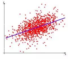
Regression algorithms attempt to explore the relationships between variables by measuring errors.Regression algorithms are powerful tools in statistical machine learning.In the field of machine learning, when people refer to regression, it sometimes refers to a type of problem and sometimes to a type of algorithm, which can often confuse beginners. Common regression algorithms include: Ordinary Least Square, Logistic Regression, Stepwise Regression, Multivariate Adaptive Regression Splines, and Locally Estimated Scatterplot Smoothing.
7. Instance-Based Algorithms
Instance-based algorithms are often used to model decision problems. Such models typically select a batch of sample data and then compare new data with sample data based on some similarity. By this method, instance-based algorithms are often referred to as “winner-takes-all” learning or “memory-based learning.” Common algorithms include k-Nearest Neighbor (KNN), Learning Vector Quantization (LVQ), and Self-Organizing Map (SOM).
8. Regularization Methods
Regularization methods are extensions of other algorithms (usually regression algorithms) that adjust the algorithms based on their complexity.Regularization methods typically reward simpler models while penalizing complex algorithms.Common algorithms include: Ridge Regression, Least Absolute Shrinkage and Selection Operator (LASSO), and Elastic Net.
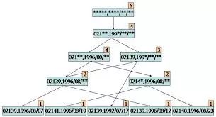
9. Decision Tree Learning
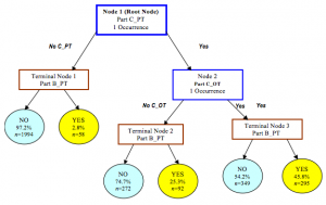
Decision tree algorithms establish decision models based on the attributes of the data using a tree structure. Decision tree models are often used to solve classification and regression problems. Common algorithms include: Classification And Regression Tree (CART), ID3 (Iterative Dichotomiser 3), C4.5, Chi-squared Automatic Interaction Detection (CHAID), Decision Stump, Random Forest, Multivariate Adaptive Regression Splines (MARS), and Gradient Boosting Machine (GBM).
10. Bayesian Methods
Bayesian methods are a class of algorithms based on Bayes’ theorem, primarily used to solve classification and regression problems. Common algorithms include: Naive Bayes, Averaged One-Dependence Estimators (AODE), and Bayesian Belief Network (BBN).
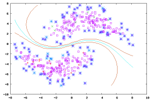
11. Kernel-Based Algorithms
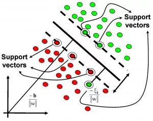
The most famous kernel-based algorithm is the Support Vector Machine (SVM). Kernel-based algorithms map input data to a higher-dimensional vector space, where some classification or regression problems can be solved more easily. Common kernel-based algorithms include: Support Vector Machine (SVM), Radial Basis Function (RBF), and Linear Discriminant Analysis (LDA).
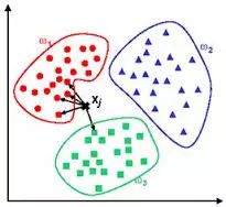
12. Clustering Algorithms
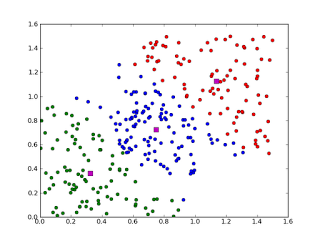
Clustering, like regression, can sometimes refer to a class of problems or a class of algorithms. Clustering algorithms typically merge input data based on central points or hierarchical methods.All clustering algorithms attempt to find the intrinsic structure of the data to classify it based on the greatest commonalities.Common clustering algorithms include k-Means and Expectation Maximization (EM).
13. Association Rule Learning
Association rule learning finds useful association rules in large multivariate datasets by searching for the rules that best explain the relationships between data variables. Common algorithms include Apriori and Eclat.
14. Artificial Neural Networks
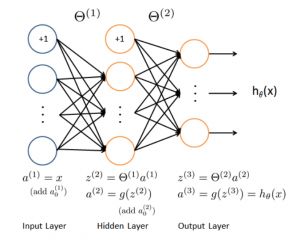
Artificial neural network algorithms simulate biological neural networks and are a class of pattern matching algorithms. They are typically used to solve classification and regression problems. Artificial neural networks are a vast branch of machine learning, with hundreds of different algorithms (including deep learning, which is a class of algorithms we will discuss separately). Important artificial neural network algorithms include: Perceptron Neural Network, Back Propagation, Hopfield Network, and Self-Organizing Map (SOM).
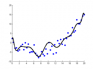
15. Deep Learning

Deep learning algorithms are an evolution of artificial neural networks. Recently, they have gained significant attention, especially after Baidu started focusing on deep learning, which has attracted a lot of attention domestically. As computational power becomes increasingly affordable, deep learning attempts to build much larger and more complex neural networks. Many deep learning algorithms are semi-supervised learning algorithms used to handle large datasets with a small amount of unlabeled data. Common deep learning algorithms include: Restricted Boltzmann Machine (RBM), Deep Belief Networks (DBN), Convolutional Networks, and Stacked Auto-encoders.
16. Dimensionality Reduction Algorithms
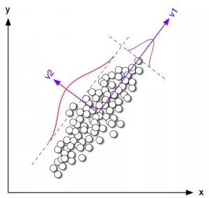
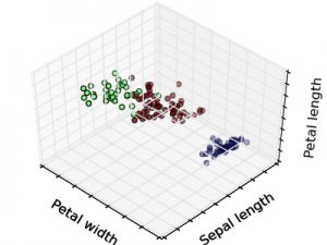
Like clustering algorithms, dimensionality reduction algorithms attempt to analyze the intrinsic structure of the data, but dimensionality reduction algorithms use unsupervised learning to generalize or explain data with less information.These algorithms can be used for high-dimensional data visualization or to simplify data for use in supervised learning.
Common algorithms include: Principal Component Analysis (PCA), Partial Least Square Regression (PLS), Sammon Mapping, Multi-Dimensional Scaling (MDS), and Projection Pursuit.
17. Ensemble Algorithms:

Ensemble algorithms train several relatively weak learning models independently on the same samples and then combine the results for overall prediction. The main difficulty with ensemble algorithms lies in determining which independent weak learning models to include and how to integrate the learning results.
This is a very powerful and popular class of algorithms. Common algorithms include: Boosting, Bootstrapped Aggregation (Bagging), AdaBoost, Stacked Generalization (Blending), Gradient Boosting Machine (GBM), and Random Forest.
Common Advantages and Disadvantages of Machine Learning Algorithms:
Naive Bayes:
1. If the lengths of the given feature vectors may differ, they need to be normalized to a common length vector (using text classification as an example), for instance, if it is sentence words, then the length is the total vocabulary length, with corresponding positions being the number of times that word appears.
2. The calculation formula is as follows:
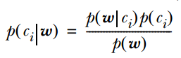
One conditional probability can be expanded through the naive Bayes conditional independence. It is important to note that  calculation method, and from the naive Bayes assumption,
 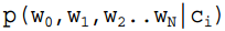 =
= , thus generally there are two methods: one is to find the total occurrence of
  in the samples of category ci, and then divide by the total of that sample; the second method is to find the total occurrence of
  in the samples of category ci, and then divide by the total occurrence of all features in that sample.
3. If any item in  is 0, then the product of the joint probability may also be 0, meaning the numerator in formula 2 is 0. To avoid this situation, generally, this item is initialized to 1, and of course, to ensure the probabilities are equal, the denominator should correspondingly be initialized to 2 (here because it is 2 classes, so add 2; if it is k classes, then it needs to add k, a term called Laplace smoothing, the reason for adding k to the denominator is to satisfy the total probability formula).
Advantages of Naive Bayes: Performs well on small-scale data, suitable for multi-class tasks, and suitable for incremental training.
Disadvantages: Sensitive to the form of input data.
Decision Trees:A key point in decision trees is selecting an attribute to branch, so it is important to pay attention to the calculation formula for information gain and to understand it deeply.
The calculation formula for information entropy is as follows:
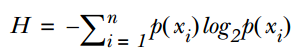
Where n represents the number of classification categories (for example, assuming a two-class problem, then n=2). Calculate the probabilities p1 and p2 of these two classes in the total sample, and thus calculate the information entropy before selecting the attribute for branching.
Now select an attribute xi to branch, where the branching rule is: if xi=vx, the sample goes into one branch of the tree; if not equal, it goes into another branch. Clearly, the samples in the branch are likely to include two categories, calculate the entropy H1 and H2 for these two branches, and calculate the total information entropy after branching H’=p1*H1+p2*H2. Therefore, the information gain ΔH=H-H’. Using information gain as a principle, test all attributes to select the one with the highest gain as the branching attribute for this time.
Advantages of Decision Trees: Simple calculation, strong interpretability, relatively suitable for handling samples with missing attribute values, can handle irrelevant features;
Disadvantages: Prone to overfitting (subsequently, Random Forest was introduced to reduce overfitting).
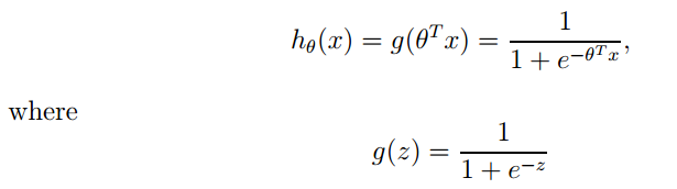
Logistic Regression:Logistic is used for classification and is a linear classifier, and key points to note include:
1. The expression for the logistic function is:
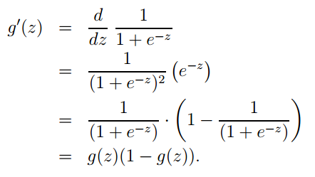
Its derivative form is:
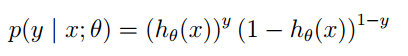
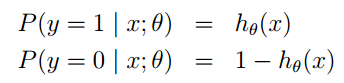
2. The logistic regression method mainly learns using maximum likelihood estimation, so the posterior probability of a single sample is:
To the posterior probability of the entire sample:
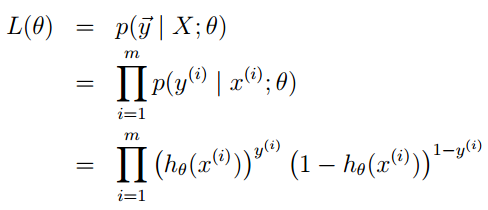
Where:
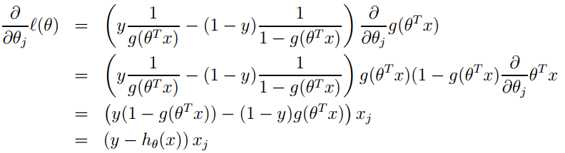
Through logarithm simplification:
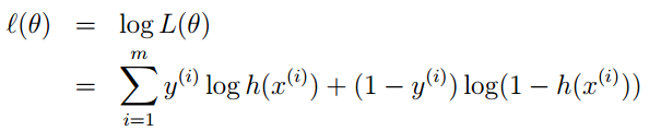
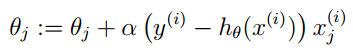
3. In fact, its loss function is -l(θ), thus we need to minimize the loss function, which can be achieved using gradient descent. The gradient descent formula is:
Logistic Regression Advantages:
1. Simple to implement
2. Very low computational cost during classification, very fast, low storage resources;
Disadvantages:
1. Prone to underfitting, generally has low accuracy
2. Can only handle binary classification problems (the derived softmax can be used for multi-class), and must be linearly separable;
Linear Regression:
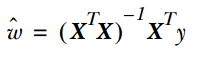
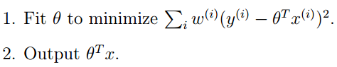
Linear regression is truly used for regression, unlike logistic regression which is used for classification. Its basic idea is to optimize the error function in the form of least squares using gradient descent, and can also directly obtain the parameter solution using the normal equation, yielding:
In LWLR (Locally Weighted Linear Regression), the parameter calculation expression is:
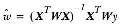
At this point, the optimization is:
It can be seen that LWLR differs from LR in that LWLR is a non-parametric model, as each regression calculation requires traversing the training samples at least once.
Linear Regression Advantages: Simple to implement, simple calculations;
Disadvantages: Cannot fit non-linear data;
KNN Algorithm:KNN, or the k-nearest neighbors algorithm, involves the following main steps:
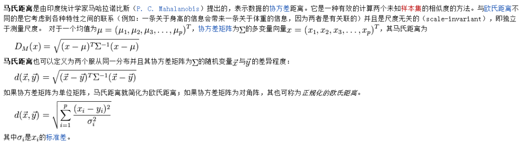
1. Calculate the distance between each sample point in the training samples and the test samples (common distance metrics include Euclidean distance, Mahalanobis distance, etc.);
2. Sort all the distance values;
3. Select the k samples with the smallest distances;
4. Based on the labels of these k samples, perform voting to obtain the final classification category;
Choosing the best K value depends on the data. Generally, a larger K value can reduce the impact of noise during classification but may blur the boundaries between categories. A good K value can be obtained through various heuristic techniques, such as cross-validation.Additionally, the presence of noise and irrelevant feature vectors can reduce the accuracy of the K-nearest neighbors algorithm.
The nearest neighbor algorithm has strong consistency results. As the data approaches infinity, the algorithm guarantees that the error rate will not exceed twice that of the Bayes algorithm error rate. For some good K values, K-nearest neighbors guarantees that the error rate will not exceed the Bayes theoretical error rate.
Note: Mahalanobis distance must first provide the statistical characteristics of the sample set, such as mean vector, covariance matrix, etc. The introduction to Mahalanobis distance is as follows:
KNN Algorithm Advantages:
1. Simple idea, mature theory, can be used for both classification and regression;
2. Can be used for non-linear classification;
3. Training time complexity is O(n);
4. High accuracy, no assumptions about the data, insensitive to outliers;
Disadvantages:
1. High computational cost;
2. Sample imbalance problem (i.e., some categories have a lot of samples while others have very few);
3. Requires a large amount of memory;
SVM:
Learn how to use libsvm and some parameter adjustment experiences, and clarify some ideas about SVM algorithms:
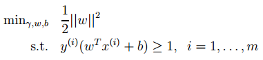
1. The optimal classification surface in SVM maximizes the geometric margin for all samples (why choose the maximum margin classifier? Please explain from a mathematical perspective; this was asked during an interview for a deep learning position at NetEase. The answer is that there is a relationship between geometric margin and the number of misclassifications of samples: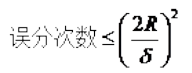 where the denominator is the distance from the sample to the classification margin, and R in the numerator is the longest vector among all samples), namely:
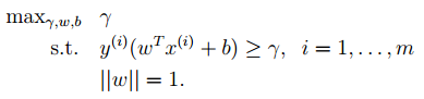
Through a series of derivations, the optimization problem can be expressed as:
2. Now let’s look at Lagrange theory:
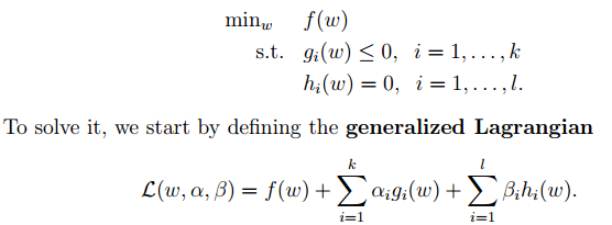
We can convert the optimization target in 1 to the Lagrangian form (through various dual optimizations, KKD conditions), and the final objective function is:
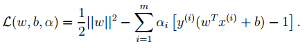
We only need to minimize the above objective function, where α is the Lagrange multiplier corresponding to the inequality constraint in the original optimization problem.
3. By taking derivatives of the last objective function in 2 with respect to w and b, we can obtain:
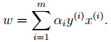
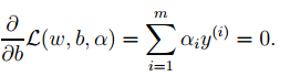
From the first formula above, we can see that if we optimize α, we can directly obtain w, which means we have determined the model parameters. The second formula can serve as a constraint condition for subsequent optimization.
4. The last objective function in 2 can be transformed into the optimization of the following objective function using dual optimization theory:
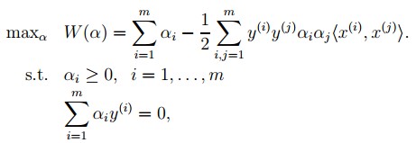
This function can be solved for α using common optimization methods, and then w and b can be obtained.
5. In principle, the simple theory of SVM should end here. However, one more point to supplement is that during prediction:
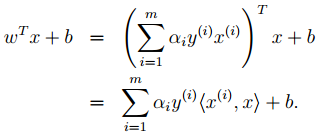
The angle brackets can be replaced with kernel functions, which is also the reason why SVM is often associated with kernel functions.
6. Finally, regarding the introduction of slack variables, the original optimization formula is:

The corresponding dual optimization formula is:
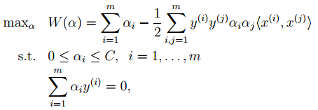
Compared to the previous one, α now has an upper bound.
Advantages of SVM:
1. Can be used for linear/non-linear classification and also for regression;
2. Low generalization error;
3. Easy to interpret;
4. Low computational complexity;
Disadvantages:
1. Sensitive to parameter and kernel function selection;
2. The original SVM is only good at handling binary classification problems;
Boosting:
Using Adaboost as an example, let’s first look at the flowchart of Adaboost:
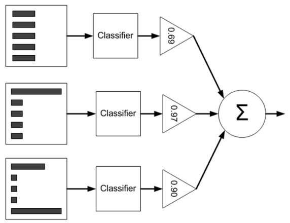
From the chart, we can see that during the training process, we need to train multiple weak classifiers (3 in the figure), each weak classifier is trained with samples of different weights (5 training samples in the figure), and each weak classifier has a different effect on the final classification result, which is output through weighted averaging. The weights are indicated by the values inside the triangle in the figure. So how are these weak classifiers and their corresponding weights trained?
Let’s illustrate this with a simple example: Suppose there are 5 training samples, each with a dimension of 2. When training the first classifier, the weights of the 5 samples are all 0.2. Note that the weight of the samples corresponds to the weights of the weak classifiers trained (α) but they are different; sample weights are only used during training, while α is used both during training and testing.
Now assume the weak classifier is a simple decision tree with one node, which will select one of the two attributes (assuming only two attributes) and calculate the best value within that attribute for classification.
Adaboost’s simple version training process is as follows:
1. Train the first classifier, the sample weights D are the same mean value. Using a weak classifier, obtain the predicted labels for these 5 samples (please refer to the example in the book, still machine learning in action) and compare with the true labels of the samples to find the error (i.e., the mistakes). If a sample is predicted incorrectly, its corresponding error value is the weight of that sample; if classified correctly, the error value is 0. Finally, sum the errors of the 5 samples to get the total error rate ε.
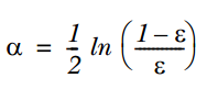
2. Calculate the weight α of that weak classifier using ε, as follows:
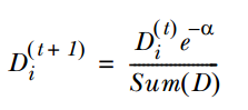
3. Use α to calculate the weights D of the samples for training the next weak classifier. If the corresponding sample is classified correctly, reduce the weight of that sample, as follows:
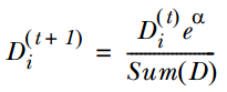
If the sample is misclassified, increase its weight, as follows:
4. Repeat steps 1, 2, and 3 to continue training multiple classifiers, just with different D values.
The testing process is as follows:
Input a sample into each trained weak classifier, and each weak classifier corresponds to an output label, then that label is multiplied by the corresponding α, and finally, the sum of the values gives the predicted label.
Advantages of Boosting Algorithms:
1. Low generalization error;
2. Easy to implement, high classification accuracy, with few parameters to adjust;
3. Disadvantages:
4. Sensitive to outliers;
Clustering:
Based on clustering ideas, we can categorize:
1. Partition-based clustering:
k-means, k-medoids (finding a sample point to represent each category), CLARANS.
k-means aims to minimize the following expression:
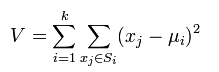
Advantages of k-means:
(1) k-means is a classic algorithm for solving clustering problems; it is simple and fast.
(2) For large datasets, this algorithm is relatively scalable and efficient, as its complexity is approximately O(nkt), where n is the number of all objects, k is the number of clusters, and t is the number of iterations. Typically, k<<n. This algorithm usually converges locally.
(3) The algorithm attempts to find k partitions that minimize the squared error function value. The clustering effect is better when the clusters are dense, spherical, or globular, and clearly distinguishable from each other.
Disadvantages:
(1) The k-means method can only be used when the average values of the clusters are defined, and it is not suitable for some categorical data attributes.
(2) The user must specify the number of clusters k to be generated in advance.
(3) Sensitive to initial values; different initial values may lead to different clustering results.
(4) Not suitable for discovering clusters of non-convex shapes or clusters with significantly different sizes.
(5) Sensitive to