
This article is the eighteenth in the “Kids Can Understand” series. The series featuresshort content that can be read in fragmented time, but the effort I put into it is substantial. If you like it, that’s enough!
-
Neural Networks That Kids Can Understand
-
Recommendation Systems That Kids Can Understand
-
Incremental Learning That Kids Can Understand
-
Clustering That Kids Can Understand
-
Principal Component Analysis That Kids Can Understand
-
Recurrent Neural Networks That Kids Can Understand
-
Embedding That Kids Can Understand
-
Entropy, Cross Entropy, and KL Divergence That Kids Can Understand
-
p-value That Kids Can Understand
-
Hypothesis Testing That Kids Can Understand
-
Gini Impurity That Kids Can Understand
-
ROC That Kids Can Understand
-
SVD That Kids Can Understand
-
SVD 2 That Kids Can Understand
-
GMM That Kids Can Understand
-
Beta Distribution That Kids Can Understand
-
Multi-Armed Bandit That Kids Can Understand
-
GAN That Kids Can Understand
0
What is GAN
The full name of GAN is Generative Adversarial Network, which in Chinese is 生成对抗网络.
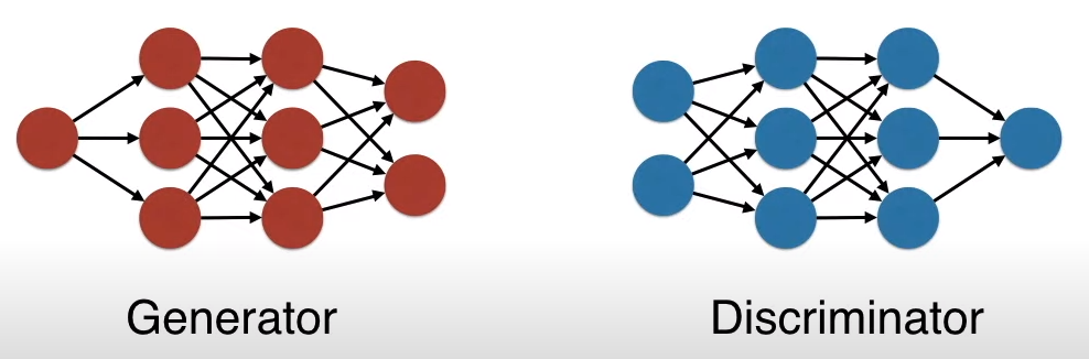
In short, GAN consists of two neural networks: the generator and the discriminator, which continuously compete with each other, with the generator producing increasingly realistic outputs and the discriminator’s recognition ability becoming more powerful.
2
Counterfeiting and Appraisal
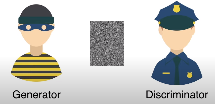
The relationship between the generator and the discriminator is similar to that of the counterfeiter and the appraiser.
-
The counterfeiter continuously produces counterfeit goods with the aim of deceiving the appraiser, and in this process, their counterfeiting skills improve.
-
The appraiser continuously examines the counterfeits with the goal of identifying the counterfeiter, and in this process, their appraisal skills improve.
GAN is both the counterfeiter and the appraiser, but ultimately, it is still the counterfeiter. The ultimate goal of GAN is to train a “perfect” counterfeiter, which can produce outputs that confuse even the appraiser.
A picture is worth a thousand words; the following image shows how the counterfeiter gradually generates a realistic Mona Lisa painting and ultimately deceives the appraiser.
In this process, whenever the counterfeiter generates an image, the appraiser provides feedback, and the counterfeiter learns how to improve to create a realistic image.
3
Counterfeit Appraisal Network?
Returning to neural networks, the counterfeiter uses the generator for modeling, while the appraiser uses the discriminator for modeling.
According to the above animation, the discriminator’s task is to distinguish which images are real and which images are produced by the generator.
Next, we will create a minimal GAN using Python.
First, let’s set a story background.
4
Story Background
On Slanted Island, everyone is slanted, probably about 45 degrees to the left.
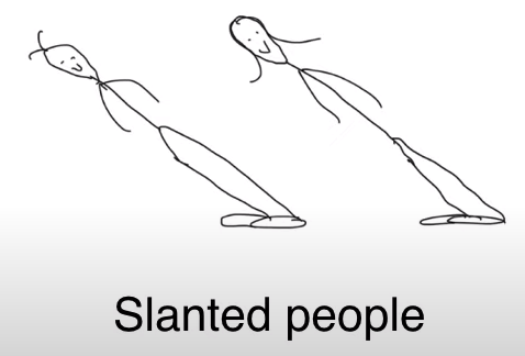
The island owner wants to create a face generator, and since the facial features of the people on the island are very simple, they use 2 * 2 pixel blurry face images.
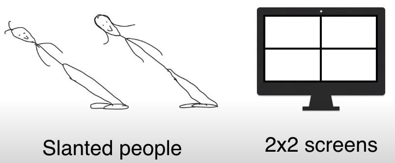
Due to technical limitations, the island owner only used a single-layer neural network.
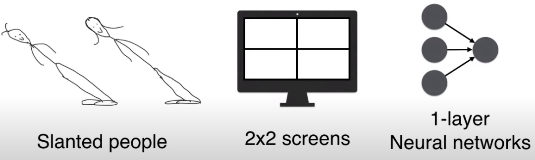
However, even in this extremely simple setup, a single-layer GAN can still generate “slanted faces”.
5
Distinguishing Faces
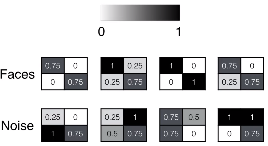
The following image shows what four faces look like.
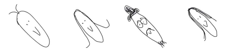
Representing faces with 2*2 pixels, dark colors indicate the presence of a face, while light colors indicate the absence of a face.
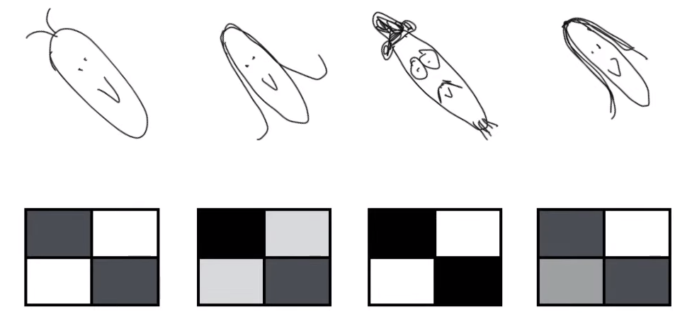
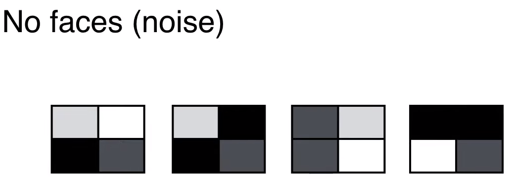
If it’s not a face? Then the elements in its 2*2 pixel image are random, as shown below.
Let’s review:
-
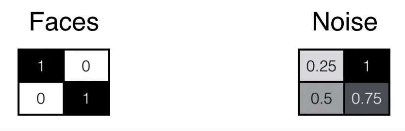
Face: Dark on the diagonal, light off the diagonal
-
Non-Face: Any area can be dark or light
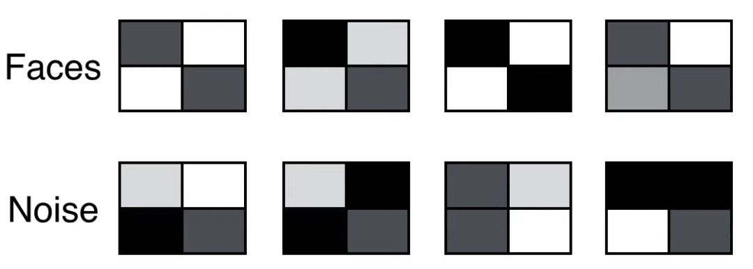
Pixels can be represented by values from 0 to 1:
-
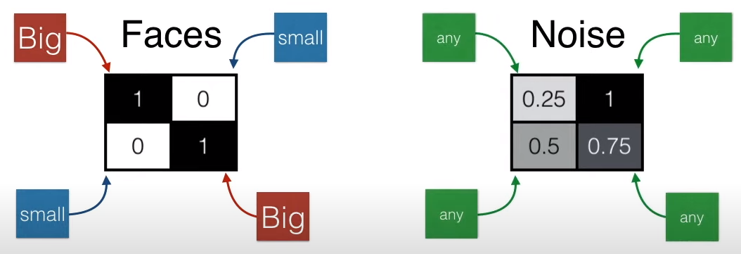
Face: Large values on the diagonal, small values off the diagonal
-
Non-Face: Any value between 0-1 can be anywhere
Having understood how facial and non-facial images are represented by different characteristic 2*2 value matrices, let’s look at how to construct the discriminator and generator in the next two sections.
First, let’s analyze the discriminator.
6
Discriminator
The discriminator is used to identify faces, so how does it distinguish when it sees the pixel values of a photo?
Simple! We have already analyzed it in the previous section:
-
Face: Large values on the diagonal, small values off the diagonal
-
Non-Face: Any value between 0-1 can be anywhere
What operation should be used to represent faces and non-faces with a single value? It’s simple, as shown in the figure below: add the element at position (1,1), subtract the element at (1,2), subtract the element at (2,1), and add the element at (2,2) to get a single value.
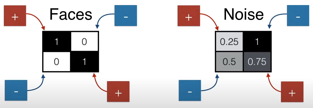
The score for a face is 2 (higher), while the score for a non-face is -0.5 (lower).
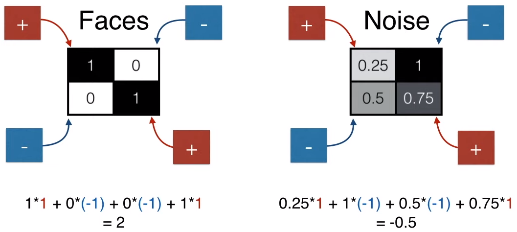
Set a threshold of 1; scores greater than 1 indicate a face, while scores less than 1 indicate a non-face.
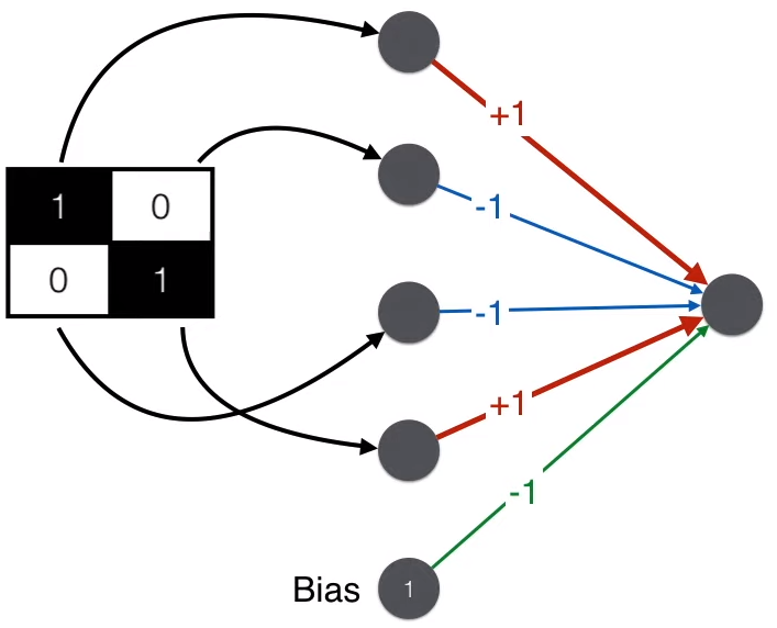
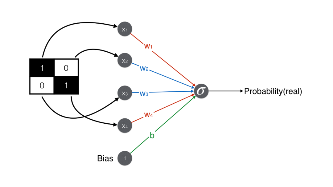
Using the above content represented in a neural network results in a minimal discriminator. Note that besides the “add-subtract-subtract-add” of the four matrix elements, a bias is also added to get the final score.
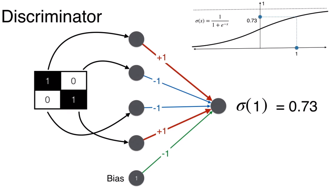
The discriminator ultimately needs to determine whether it is a face, so the output is a probability that needs to be converted from the score of 1 using the sigmoid function to a probability of 0.73. Given a probability threshold of 0.5, since 0.73 > 0.5, the discriminator judges that the image is a face.
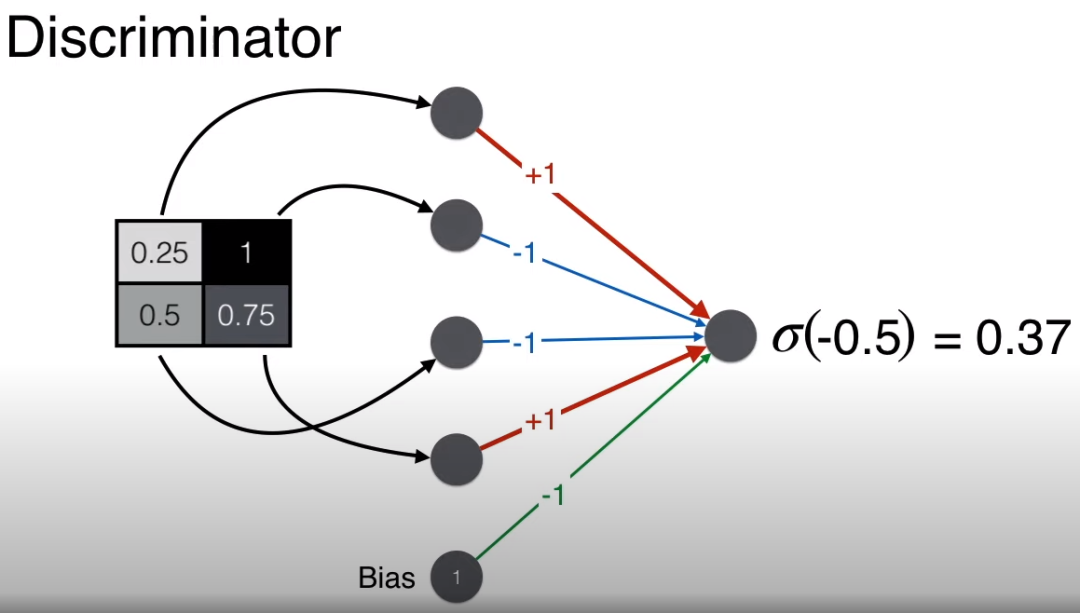
For another non-face image, using the same operation, the final score is calculated as -0.5. After applying the sigmoid function, given a probability threshold of 0.5, since 0.37 < 0.5, the discriminator judges that the image is a face.
7
Generator
The discriminator aims to identify faces, while the generator aims to generate faces. So, what kind of matrix pixels resemble a face? Simple! The rules have been analyzed multiple times:
-
Face: Large values on the diagonal, small values off the diagonal
-
Non-Face: Any value between 0-1 can be anywhere

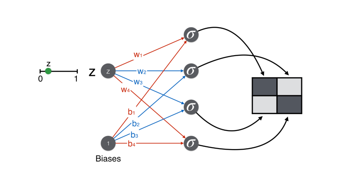
Now let’s look at the generation process. The first step is to randomly select a number between 0-1, for example, 0.7.
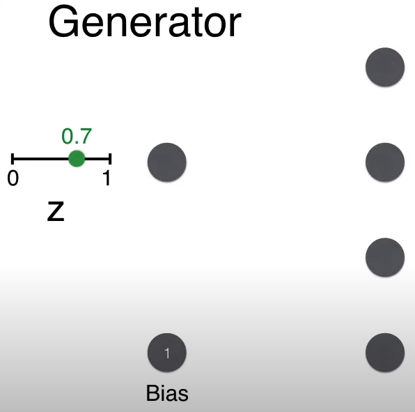
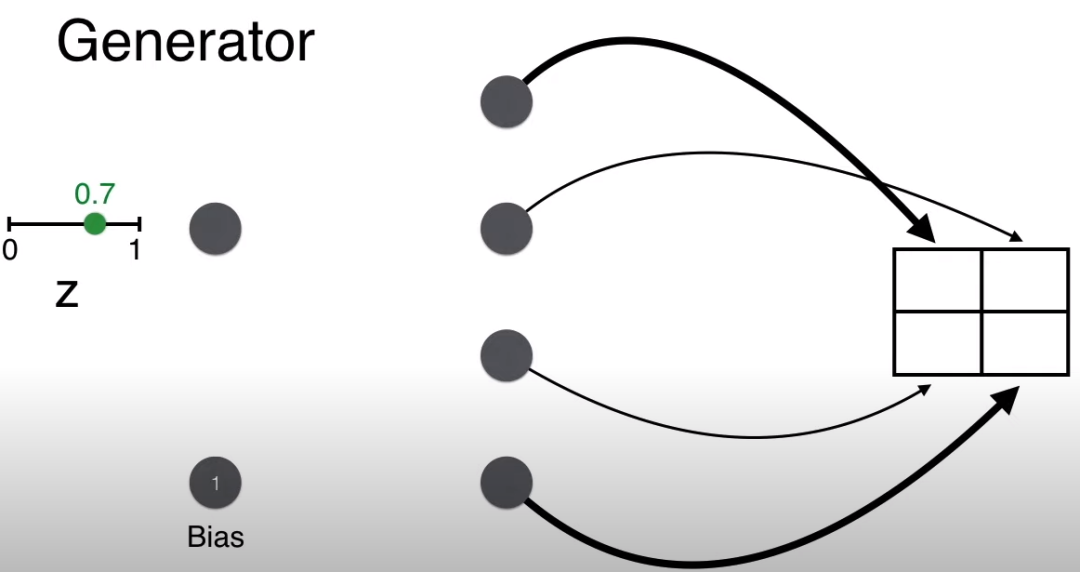
Recall that the generator’s goal is to generate faces, meaning that the final 2*2 matrix must have large pixel values on the diagonal (indicated by thick lines) and small pixel values off the diagonal (indicated by thin lines).
For example, generating the value at matrix position (1,1), with w = 1, b = 1, the calculation gives wz + b = 1.7.
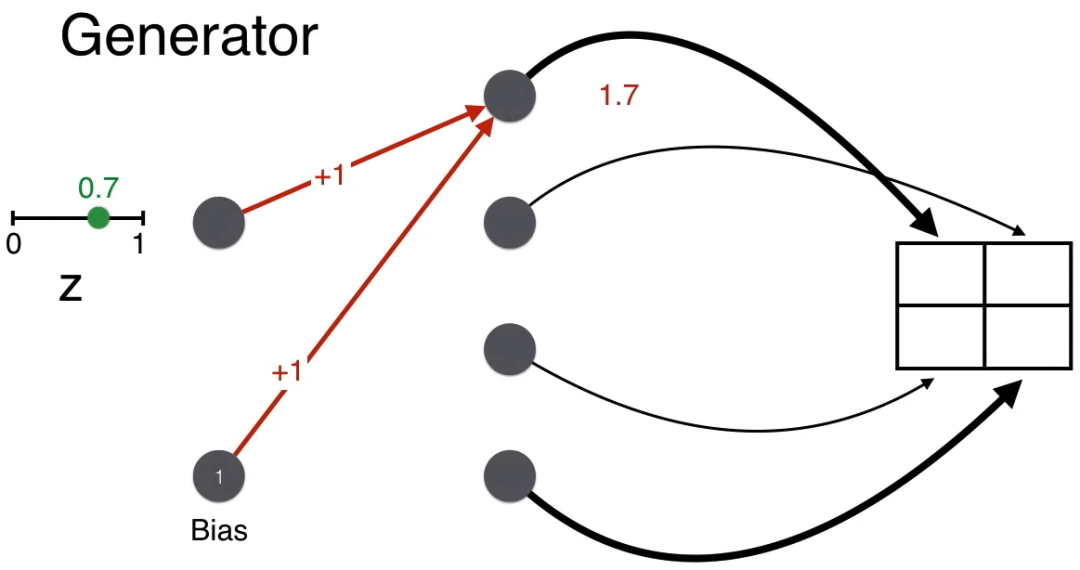
Similarly, calculate the scores for the other three positions in the matrix.
Finally, apply the sigmoid function to convert the scores, ensuring the pixel values are between 0-1.
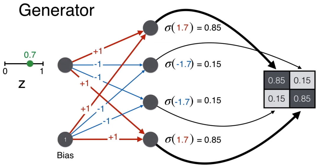
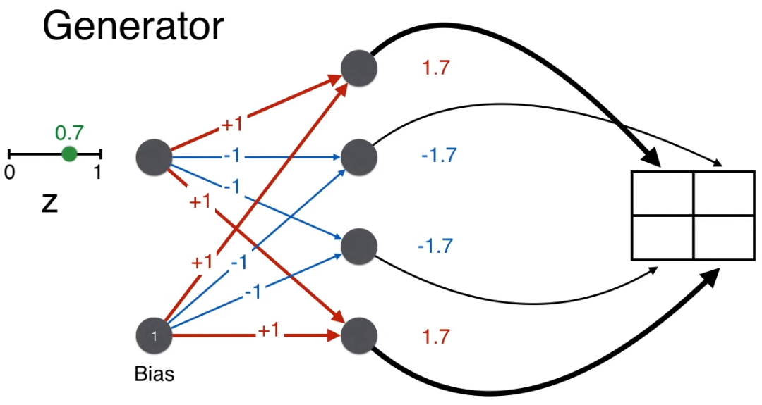
Note that by giving weights [1, -1, -1, 1] and a bias of 1, since z is always a positive number between 0 and 1, such a neural network (the generator) can always generate a 2*2 pixel matrix that resembles a face.
From the previous and this section, we now know what kind of discriminator can identify faces and what kind of generator can generate good faces, meaning what kind of GAN is a good GAN. These are determined by weights and biases; next, let’s see how they are trained. First, let’s review the error function.
8
Error Function
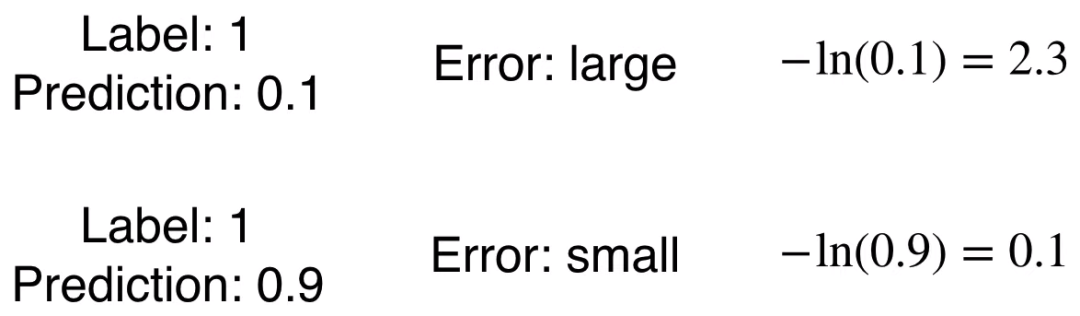
Typically, positive classes are represented by 1 and negative classes by 0. In this case, faces are positive, represented by 1; non-faces are negative, represented by 0.
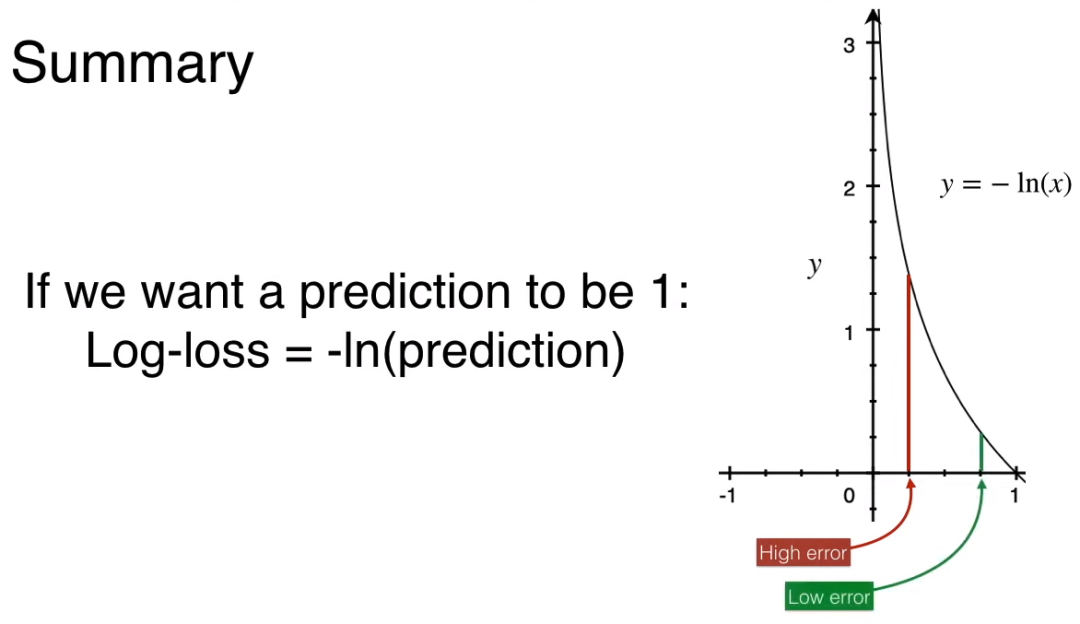
When the label is 1 (face), -ln(x) serves as a good error function because
-
When the prediction is inaccurate (predicting a non-face, say 0.1), the error should be large, -ln(0.1) is large.
-
When the prediction is accurate (predicting a face, say 0.9), the error should be small, -ln(0.9) is small.
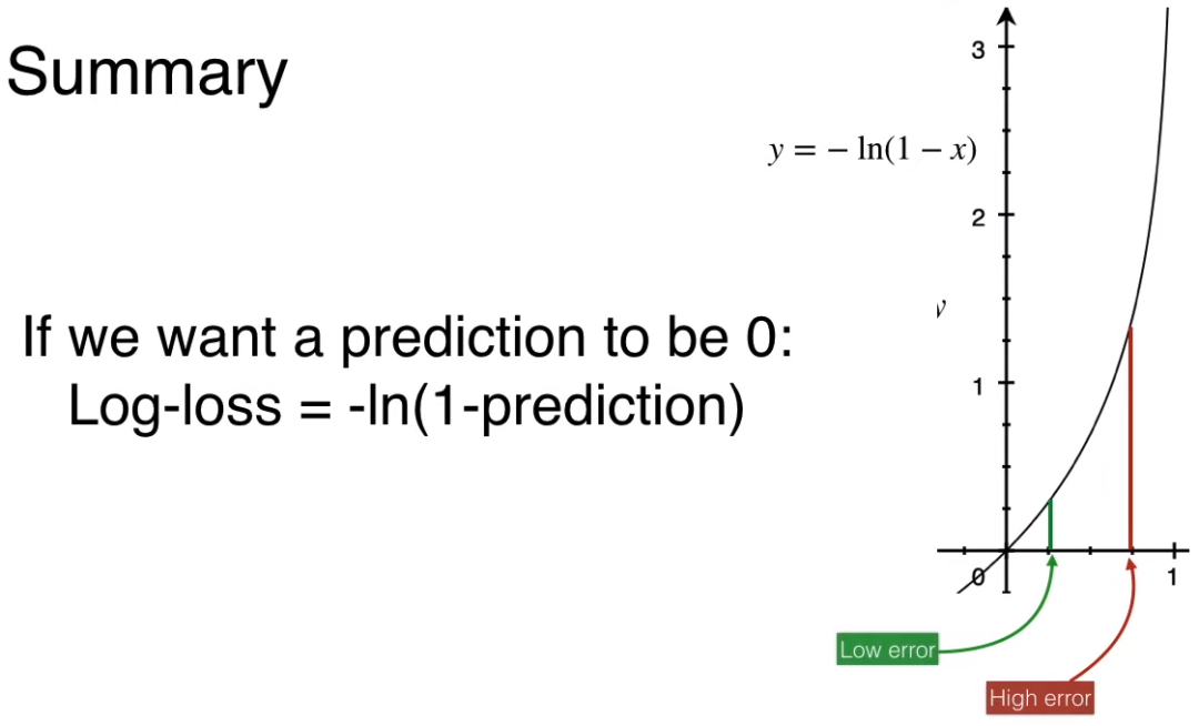
When the label is 0 (non-face), -ln(1-x) serves as a good error function.
-
When the prediction is accurate (predicting a non-face, say 0.1), the error should be small, -ln(1-0.1) is large.
-
When the prediction is inaccurate (predicting a face, say 0.9), the error should be large, -ln(1-0.9) is small.
Next is the game between GAN, where the generator and discriminator are put together to see what happens.
9
Putting the Generator and Discriminator Together
Let’s review the structure of both:
-
Generator: Input is a random number between 0-1, output is a pixel matrix of the image
-
Discriminator: Input is a pixel matrix of the image, output is a probability value

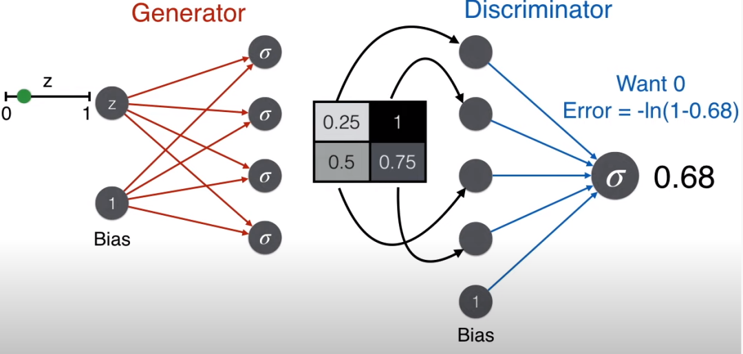
The following animation shows the process from generator to discriminator.

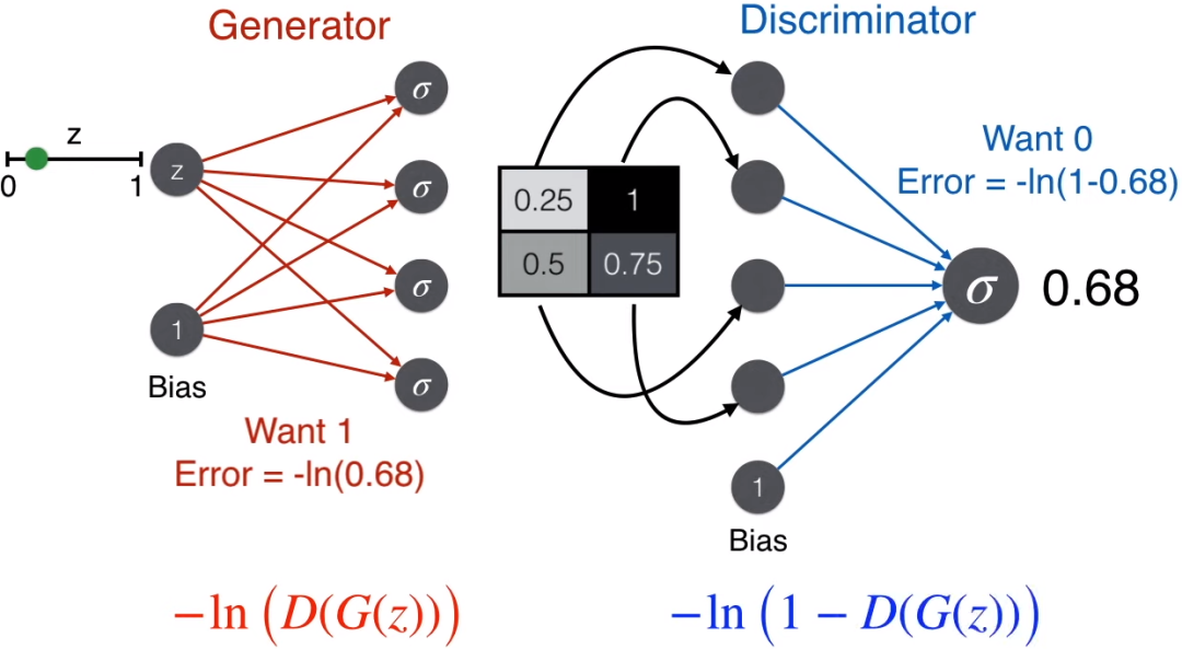
Since the image is generated from the generator and is not a real image, a good discriminator will judge that this is not a face, thus using the error function corresponding to the label of 0, -ln(1-prediction).
Conversely, a good generator aims to deceive the discriminator, i.e., it wants the discriminator to judge that this is a face, so it uses the error function corresponding to the label of 1, -ln(prediction).
Here comes the interesting part: let G represent the generator and D represent the
, then
-
G(z) is the output of the generator, i.e., the pixel matrix, which is also the input of the discriminator
-
D(G(z)) is the output of the discriminator, i.e., the probability, which is also the prediction in the error function above
To make both the generator and discriminator stronger, we want to minimize the error function
-ln(D(G(z)) – ln(1-D(G(z))
where D(G(z)) is the prediction of the discriminator.
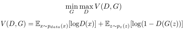
Comparing the error function we obtained with the objective function in the GAN paper (shown below), we find some differences:
Explanation as follows:
The discriminator not only receives images produced by the generator G(z), but also receives real images x. In this case, a good discriminator will judge that this is a face, thus using the error function corresponding to the label of 1, -ln(-prediction). Therefore, for the discriminator, the error function to minimize is
-ln(D(x)) – ln(1-D(G(z))
Removing the negative sign is equivalent to maximizing
ln(D(x)) + ln(1-D(G(z))
This is exactly V(D,G), right? This process fixes the generator to optimize the
After maximizing V(D, G), while fixing the
Finally, both terms in V(D, G) have expectation symbols, and in actual optimization, we achieve this through statistical averages over n samples. The x in the first term’s expectation comes from the real data distribution p_data(x), and the z in the first term’s expectation comes from a specific probability distribution p_z(z).
In summary, first maximize V(D,G) through D, then minimize V(D, G) through G.
10
Training GAN
During training, when the face comes from the generator, the discriminator outputs a probability value close to 0 by minimizing the error function.
When the face comes from a real image, the discriminator outputs a probability value close to 1 by minimizing the error function.
Of course, all neural network training algorithms are based on gradient descent.
OK, the following content is indeed not suitable for ordinary kids, but kids with a strong interest in mathematics and programming can continue reading  .
.
11
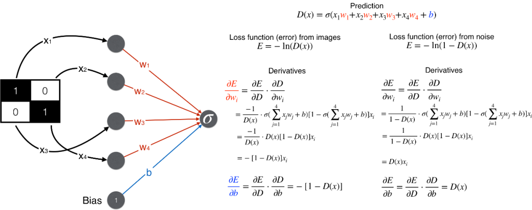
Mathematical Derivation
Discriminator: From pixel matrix to probability
Generator: From random number z to pixel matrix
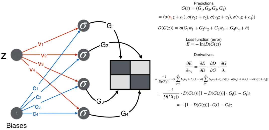
After obtaining the partial derivatives of the error function with respect to the weights and biases in the generator and discriminator, we can write the code to implement it.
12
Python Implementation – Preparation
Import numpy and matplotlib.
import numpy as npfrom numpy import randomfrom matplotlib import pyplot as plt%matplotlib inlineWrite a function to draw facial pixels.
def view_samples(samples, m, n): fig, axes = plt.subplots(figsize=(10, 10), nrows=m, ncols=n, sharey=True, sharex=True) for ax, img in zip(axes.flatten(), samples): ax.xaxis.set_visible(False) ax.yaxis.set_visible(False) im = ax.imshow(1-img.reshape((2,2)), cmap='Greys_r') return fig, axesDraw four faces, noting that the pixel matrix has large values on the diagonal and small values off the diagonal.
faces = [np.array([1,0,0,1]), np.array([0.9,0.1,0.2,0.8]), np.array([0.9,0.2,0.1,0.8]), np.array([0.8,0.1,0.2,0.9]), np.array([0.8,0.2,0.1,0.9])] _ = view_samples(faces, 1, 4)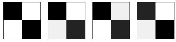
Draw twenty non-faces, noting that the pixel matrix elements are all random.
noise = [np.random.randn(2,2) for i in range(20)]def generate_random_image(): return [np.random.random(), np.random.random(), np.random.random(), np.random.random()]_ = view_samples(noise, 4,5)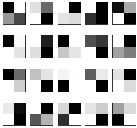
13
Python Implementation – Building the Discriminator
First, implement the sigmoid function.
def sigmoid(x): return np.exp(x)/(1.0+np.exp(x))Using object-oriented programming (OOP) to write the discriminator, the code is as follows:
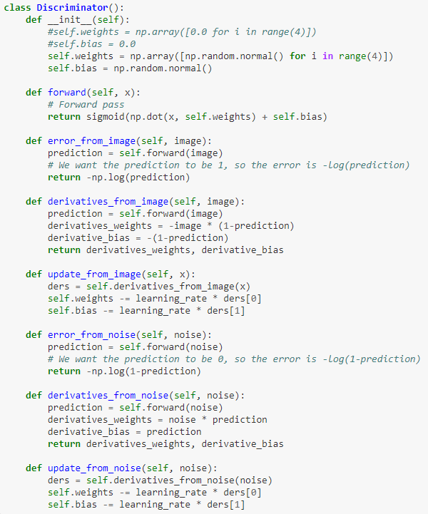
Where
-
__init__() is the constructor
-
forward() function flattens the pixel matrix into a vector x, multiplies it by weight w, adds bias b to get a score, and then converts it to probability using the sigmoid() function
-
error_form_image() calculates the error function when receiving real images as input
-
error_form_noise() calculates the error function when receiving the generator as input
-
derivatives_form_image() calculates the partial derivatives of the error function with respect to weights w and bias b when receiving real images as input
-
derivatives_form_noise() calculates the partial derivatives of the error function with respect to weights w and bias b when receiving the generator as input
-
update_form_image() calculates the gradient descent method when receiving real images as input
-
update_form_noise() calculates the gradient descent method when receiving the generator as input
14
Python Implementation – Building the Generator
Using object-oriented programming (OOP) to write the generator, the code is as follows:
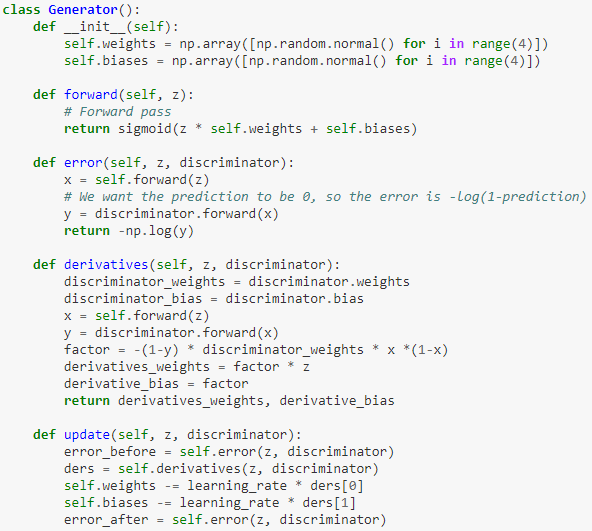
Where
-
__init__() is the constructor
-
forward() function multiplies the random number z by weight w, adds bias b to get a score, and then converts it to pixel using the sigmoid() function
-
error() calculates the error function when fixing the discriminator as input, in two steps:
-
The generator’s forward() function gets the pixels
-
The discriminator’s forward() function gets the probability
-
derivatives() calculates the partial derivatives of the error function with respect to weights w and bias b when fixing the discriminator as input, referring to the mathematical formulas in the previous section
-
update() calculates the gradient descent method when fixing the discriminator as input
15
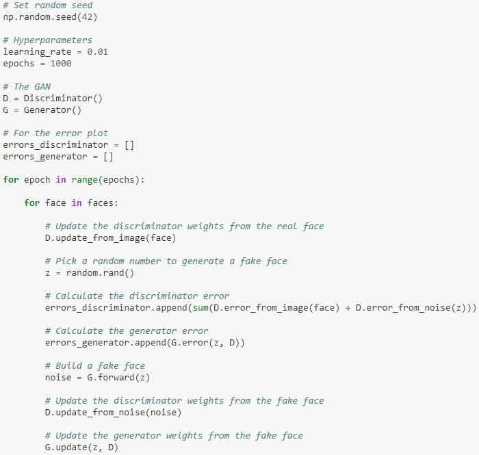
Python Implementation – Training GAN
Set 1000 epochs, meaning the data will be traversed 1000 times to start training, recording the errors of both the generator and discriminator for each epoch.
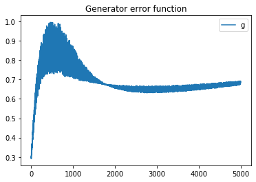
Plot the error function graph for the generator and discriminator, finding that the generator gradually stabilizes.
plt.plot(errors_generator)plt.title("Generator error function")plt.legend("gen")plt.show()plt.plot(errors_discriminator)plt.legend('disc')plt.title("Discriminator error function")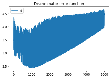
16
Python Implementation – Result Display
Generate images.
generated_images = []for i in range(4): z = random.random() generated_image = G.forward(z) generated_images.append(generated_image)_ = view_samples(generated_images, 1, 4)for i in generated_images: print(i[0.94688171 0.03401213 0.04080795 0.96308679] [0.95653992 0.03437852 0.03579494 0.97063836] [0.95056667 0.03414339 0.03893305 0.96599501] [0.94228203 0.03386046 0.04309146 0.95941292]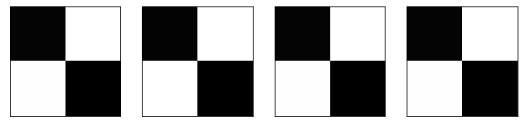
Print the final parameters of the GAN, i.e., the weights and biases of the generator and discriminator.
print("Generator weights", G.weights)print("Generator biases", G.biases)print("Discriminator weights", D.weights)print("Discriminator bias", D.bias)Generator weights [ 0.70702123 0.03720449 -0.45703394 0.79375751] Generator biases [ 2.48490157 -3.36725912 -2.90139211 2.8172726 ] Discriminator weights [ 0.60175083 -0.29127513 -0.40093314 0.37759987] Discriminator bias -0.8955103005797729Here is the GAN with weights and biases shown.
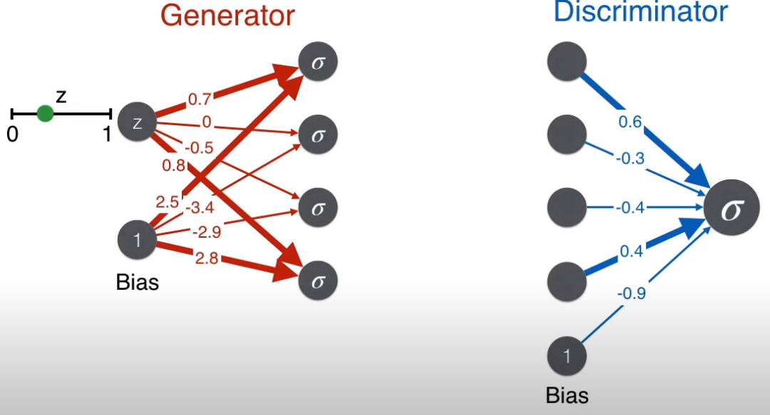
The bold lines in the figure correspond to large weights, while the thin lines correspond to small or negative weights. Comparing with the earlier goal of the generator to generate realistic faces (i.e., large values on the diagonal of the 2*2 matrix), isn’t this weight reasonable?
Friends, have you understood GANs?
If you want to learn Python content, you can refer to my “Three Sets of Python Premium Courses”.