Understanding Diffusion Models: A Unified Perspective

This article is a summary of some technical blogs and overviews that the author has recently read about diffusion models. The main reference content comes from Calvin Luo’s paper, aimed at readers who already have a basic understanding of diffusion models. Calvin Luo’s paper provides a unified perspective for understanding diffusion models, especially the detailed mathematical derivations. This article will attempt to briefly summarize the derivation process of diffusion models from a unified perspective. At the end, the author includes some thoughts and questions regarding strong assumptions in the derivation process, and briefly discusses some considerations when applying diffusion models in natural language processing.

This reading note references the following technical blogs. Readers who do not understand diffusion models may consider reading Lilian Weng’s popular science blog first. Calvin Luo’s introductory paper has been reviewed by Jonathan Ho (author of DDPM), Dr. Song Yang, and a series of authors of related diffusion model papers, making it highly recommended.

1. What are Diffusion Models? by Lilian Weng

2. Generative Modeling by Estimating Gradients of the Data Distribution by Song Yang

3. Understanding Diffusion Models: A Unified Perspective by Calvin Luo

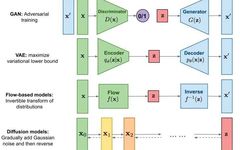
Generative models aim to generate data that conforms to the real distribution (or a given dataset). Common types of generative models include GANs, Flow-based Models, VAEs, Energy-Based Models, and the diffusion models we hope to discuss today. Diffusion models have some connections and differences with Variational Autoencoders (VAEs) and Energy-Based Models (EBMs), which will be elaborated in the following sections.

Before introducing diffusion models, let’s first review Variational Autoencoders (VAEs). We know that the biggest feature of VAEs is the introduction of a latent vector distribution to assist in modeling the real data distribution. So why do we introduce latent vectors? There are two intuitive reasons: one is that directly modeling high-dimensional representations is very difficult and often requires strong prior assumptions, and there is also the issue of the curse of dimensionality. The other is that directly learning low-dimensional latent vectors serves to compress dimensions while also hoping to explore semantic structural information in low-dimensional space (for example, in the field of images, GANs often influence specific features of output images by manipulating specific dimensions).

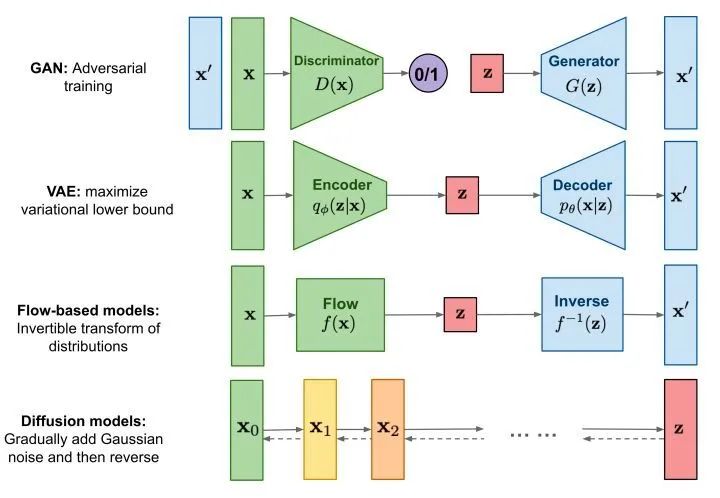
After introducing latent vectors, we can write the log-likelihood of our target distribution logP(x), also known as the “evidence,” in the following form:

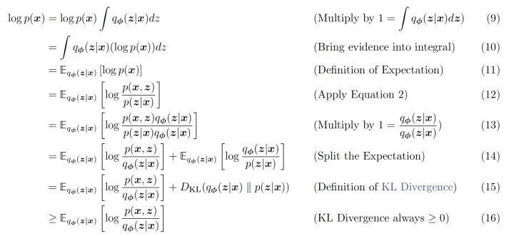
Here, we focus on equation 15. The left side of the equation is the real data distribution (evidence) that the generative model aims to approach, while the right side consists of two terms. The second term’s KL divergence is always greater than zero, so the inequality always holds. If we subtract this KL divergence from the right side of the equation, we obtain the lower bound of the real data distribution, known as the Evidence Lower Bound (ELBO). By further expanding ELBO, we can obtain the optimization objective of VAE.

We can intuitively understand the form of this lower bound: the evidence lower bound is equivalent to a process where we use an encoder to encode the input x into a posterior latent vector distribution q(z|x). We hope this vector distribution is as similar as possible to the real latent vector distribution p(z), so we use KL divergence as a constraint, which also helps to avoid the learned posterior distribution q(z|x) collapsing into a Dirac delta function (the right side of equation 19). The obtained latent vector is then reconstructed into the original data using a decoder, corresponding to the left side of equation 19 P(x|z).

Why is VAE called a variational autoencoder? The variational part comes from the process of finding the optimal latent vector distribution q(z|x). The autoencoder part refers to the encoding of the input data and the reconstruction of the original data.

So, to summarize why VAE can fit the original data distribution well: based on the above formula derivation, we find that the log-likelihood of the original data distribution (referred to as evidence) can be written as the evidence lower bound plus the KL divergence between the posterior latent vector distribution we wish to approximate and the true latent vector distribution (i.e., equation 15). If we write this as A = B+C, since evidence (i.e., A) is a constant (independent of the parameters we want to learn), maximizing B, which is our evidence lower bound, is equivalent to minimizing C, which is the difference between the distribution we wish to fit and the true distribution. Because of the evidence lower bound, we can rewrite it in the form of equation 19, which gives us the training objective of the autoencoder. Optimizing this objective is equivalent to approximating the true data distribution and is also equivalent to the process of optimizing the posterior latent vector distribution q(z|x) using variational methods.

However, VAE still has many issues. One of the most obvious is how to choose the posterior distribution q_phi(z|x). In the vast majority of VAE implementations, this posterior distribution is chosen to be a multi-dimensional Gaussian distribution. But this choice is more for computational and optimization convenience. Such a simple form greatly limits the model’s ability to approximate the true posterior distribution. The original authors of VAE, Kingma, had a very classic work that improved the expressiveness of the posterior distribution by introducing normalization flow. Diffusion models can also be seen as an improvement of the posterior distribution q_phi(z|x).

The following diagram shows a closed-loop relationship between the latent vector and the input in a variational autoencoder. That is, after extracting the low-dimensional latent vector from the input, we can reconstruct the input from this latent vector.

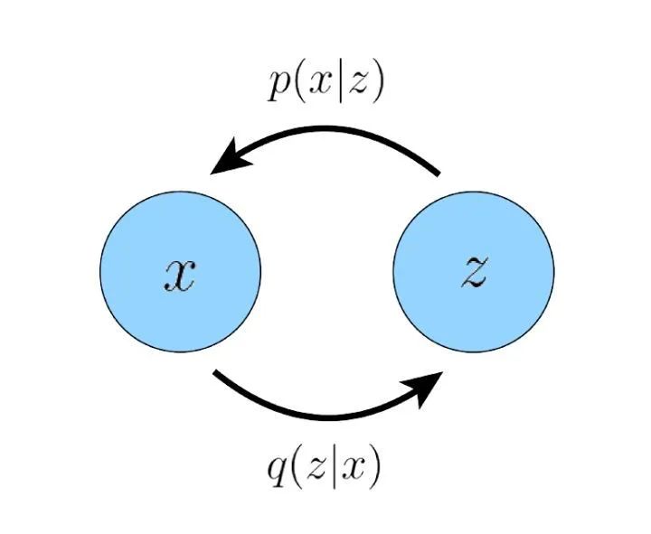
It is clear that we believe this low-dimensional latent vector must efficiently encode some important characteristics of the original data distribution for our decoder to successfully reconstruct various data from the original data distribution. So if we recursively compute the