
Introduction
• The explicit method is a true dynamic process. It was originally used to simulate high-speed collision problems.• It is used to solve the dynamic equilibrium state of structures.• During the solving process, inertial forces play a decisive role.• Unbalanced forces propagate in neighboring elements in the form of stress waves.• The stable time increment is generally small.• The explicit dynamics method can also simulate quasi-static problems, such as metal forming processes, but requires special considerations:• If calculated using natural time periods, it is impractical to solve quasi-static problems with explicit dynamics methods. Generally, millions of time increments are needed.  • To save computation time, the speed of the rolling process can be artificially increased during the simulation.• After increasing the rolling speed, the static equilibrium problem evolves into a dynamic equilibrium problem. The influence of inertial forces will increase.• The goal of quasi-static analysis is to minimize the computational time cycle while keeping the impact of inertial forces small.
Load Rate
• It is necessary to artificially increase the speed of the quasi-static forming process during the simulation, which can make the solving process more economical.• However, without degrading the results, how much can the speed be increased?• For example, in the metal forming process, the typical tool speed is about the order of 1 m/s.• This wave speed is very small compared to the typical wave speed in metals (the wave speed in steel is 5000 m/s).• The generally recommended load rate is 1% of the wave speed in the material.• Recommended methods:• Simulate multiple times at different rates (for example, tool speeds of 100, 50, 5 m/s).• Since the analysis time at low load rates is longer, analyze from high load speeds to low load speeds.• Check the results (deformation shapes, stress, strain, energy), analyze the impact of different load rates on the results.• In explicit sheet metal forming simulations, excessively high tool speeds will suppress wrinkling phenomena and provoke unrealistic localized stretching.• In buckling forming processes, excessively high tool speeds will cause the “jetting” effect—hydrodynamic response (illustrated on the next page).Jetting• Consider the following buckling forming process (cross-section of an axisymmetric model at 180°).• When the tool speed is very high, highly localized deformations occur (jetting). 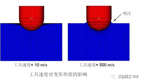 • Example: Sheet Metal• The right image shows a simplified model of the impact test of a standard door beam for a car.• The circular beam is fixed at each end and deforms after contacting a rigid circular cylinder.• The test is quasi-static.
 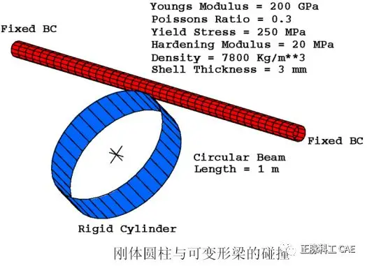 • If the collision speed is very high, 400 m/sec, the deformation is highly localized, and the beam has no structural response.• The main response in static tests is the first mode of the beam. The frequency of this mode is used to estimate the collision speed.• The first frequency is approximately 250 Hz.• The collision is completed within 4 microseconds.• Using a collision speed of 25 m/sec, the cylinder pushes the beam 0.1 m in 4 microseconds.
 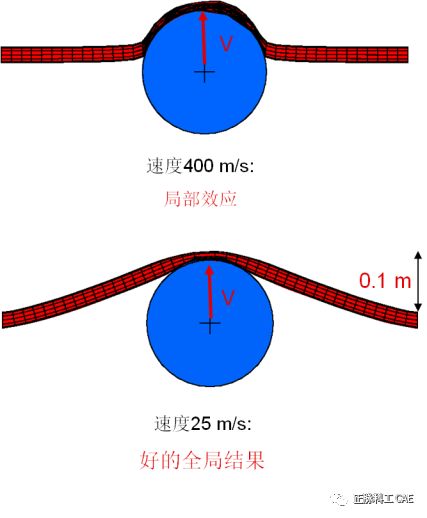 • Why is a speed of 25 m/sec appropriate?• The first frequency (f) is approximately 250 Hz.• The corresponding period is t=0.004 seconds.• Within this period, the rigid circular cylinder is pushed towards the beam d = 0.1 m.• Thus, the estimated speed v is v = d/t = 0.1/0.004 = 25 m/sec.• The metal wave speed is 5000 m/sec, so the collision speed of 25 m/sec is 0.5% of the wave speed.• The collision speed should be less than 1% of the material wave speed.• During the analysis step, increasing the collision speed from zero to the applied collision speed in a smooth ramp manner can yield more accurate solutions.• SMOOTH STEP amplitude curve• By gradually applying the load, the accuracy of the quasi-static solution can be improved:• Constant speed conditions in the tool lead to sudden impact loads on the metal blank.• This will cause stress waves to pass through the blank, resulting in undesirable outcomes.• By gradually increasing the tool speed from zero in a ramp manner, these adverse effects can be reduced.• For the same reason, during the process of removing the tool at the end of the analysis, the tool speed should also be gradually decreased to zero in a ramp manner.SMOOTH STEP amplitude defines a transition between two amplitudes with a 5th order polynomial. For example, the first and second time derivatives are zero at the start and end of the transition.When using SMOOTH STEP to define the displacement time history, the velocity and acceleration at each specified amplitude are zero.*AMPLITUDE, NAME=SSTEP, DEFINITION=SMOOTH STEP0.0, 0.0, 1.0E-5, 1.0*BOUNDARY, TYPE=DISPLACEMENT, AMP=SSTEP12, 2, 2, 2.5
Energy Balance
• The energy balance equation can be used to help evaluate whether the computational results are a reasonable quasi-static response.• In Abaqus/Explicit, the energy balance can be written as where EKE is the kinetic energy. EI is the internal energy (including elastic strain energy, plastic strain energy, and pseudo energy related to hourglass control). EV is the energy dissipated by viscous mechanisms. EFD is the energy dissipated by friction. EW is the work done by external forces. ETOT is the total energy of the system.• Consider the tensile test of a uniaxial tensile specimen.• If the actual test is quasi-static, the external work done on the tensile specimen equals the internal energy of the specimen.  • The energy history of the quasi-static test is shown in the right image:• Inertial forces can be neglected.• The material speed of the test specimen is very small.• The kinetic energy can be neglected.• As the speed of the test increases:• The response of the specimen deviates from static and trends towards dynamic.• Therefore, the material speed and kinetic energy become more pronounced.
  • Therefore, energy checks provide another method for evaluating whether the results of the Abaqus/Explicit metal forming process reflect a quasi-static solution.• In the main forming process, the kinetic energy of the deformed material should not exceed a small portion of the internal energy.• This small portion is generally 1–5%.• Because the blank will be moved before significant deformation occurs, it is generally difficult to reach this value early in the forming process.• Using smooth amplitude curves will improve early responses. • The kinetic energy of the tool is not of concern.• Subtract the kinetic energy of the tool from the total kinetic energy of the model, or limit the energy output of the deforming component.• Example: Deep drawing of a cylindrical cup.• The right image shows a 1/4 model of the finite element model.• Friction is defined at all contact surfaces:• Punch and blank: m = 0.25.• Die and blank: m = 0.125.• Blank holder and blank: m = 0.• The deep drawing process is simulated by applying a downward force of 22.87 KN on the blank holder and moving the punch down by 36 mm.
 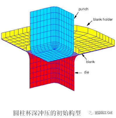 • Try three different stamping speeds:• 3 m/s• 30 m/s• 150 m/s• The table below summarizes the computational costs for each deep drawing of the cylindrical cup:
 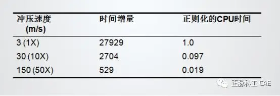 • The final configuration shows the thickness cloud of the blank.• Excessively high stamping speeds lead to results that do not align with actual physical phenomena.• Despite the computational costs differing by a factor of 10, the results of stamping at speeds of 30 m/s and 3 m/s are very close.
 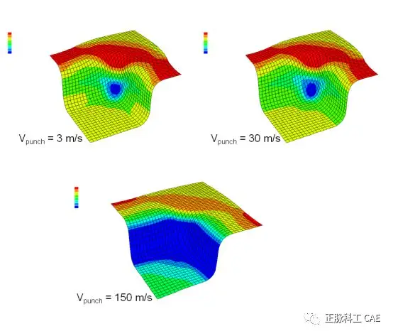 • Comparing internal energy and kinetic energy• When the stamping speed is 150 m/s, the kinetic energy in the blank occupies a large proportion compared to the internal energy.• When the stamping speeds are 3 m/s and 30 m/s, the kinetic energy occupies only a small part compared to the internal energy during the forming process.
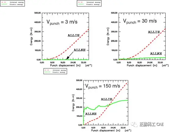
Mass Scaling
• Artificially increasing the forming speed can improve the economic efficiency of the solution. At the same time, the material strain rate increases at the same speed.• If the material is strain rate insensitive, this is irrelevant.• If strain rate sensitivity is considered in the model, it will lead to erroneous results.• If rate dependency is considered, it generally requires simulating the forming process using natural time periods.• This functionality can be achieved through mass scaling.• The estimated formula for the stability limit of explicit dynamic processes is 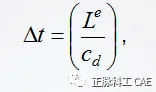 where Le is the minimum feature element length, cd is the material expansion wave speed.• The Poisson’s ratio is• The material expansion wave speed is
 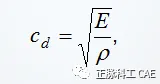 where E is Young’s modulus, r is the material density.• If the material density is artificially increased by f^2:• The expansion wave speed decreases by f.• The stability time increment increases by f.• By artificially increasing the stability time through mass scaling, it allows for the analysis of the forming process using natural time periods.• After artificially increasing the tool speed, mass scaling has the same effect on inertial effects. Excessive mass scaling will lead to unrealistic solutions.• If mass scaling is used under fully dynamic conditions, the total mass change should be kept as small as possible (less than 1%).• The *FIXED MASS SCALING option can be used for mass scaling. *FIXED MASS SCALING applies mass scaling at the start of the analysis step.• Syntax:*FIXED MASS SCALING, ELSET=name, FACTOR= f^2 • In the corresponding element set, the density of each element increases by f^2, thus increasing the stability time increment by f.• Example of mass scaling:• The right image shows the tensile test of a low-carbon steel plane strain specimen.• Due to symmetry, only 1/4 of the model is selected.
  • The graphics show the different results of three analyses (PEEQ cloud diagram)• The results on the left and the middle in the right image are almost the same.• The middle result requires only 1/5 of the computation time compared to the left result.• The right result is essentially meaningless compared to the original static solution.
Mesh Adaptation
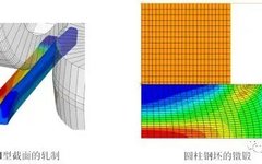
• Purpose• In many nonlinear simulations, materials in structures or processing undergo very large deformations.• These deformations will distort the finite element mesh, and overly distorted meshes will not yield accurate solutions or may cause the analysis to terminate prematurely due to numerical reasons.• In these simulations, mesh adaptation tools must be used to periodically reduce mesh distortion.• Note: In this lecture, we only discuss the ALE adaptive mesh in Explicit; the adaptive mesh format in Standard will be mentioned in future lectures.• Mesh adaptation is useful for many problems:• For transient problems with large deformations, it can be used as a continuous adaptive mesh tool. For example:• Dynamic impact• Penetration• Oscillation• Forging• It can also be used as a solution technique to simulate steady-state processes, such as:• Extrusion• Rolling• As a tool, it can analyze instantaneous states in steady-state processes.• Basics of Mesh Adaptation• In Abaqus/Explicit, the adaptive mesh function is implemented through arbitrary Lagrangian-Eulerian (ALE) methods. The basic features of the adaptive mesh function are:• The mesh is regularly smoothed to reduce element distortion and maintain good aspect ratios of the elements.• The original topological relationship of the mesh is preserved—element numbers, node numbers, and their connectivity do not change.• It can analyze Lagrangian (transient) problems and Eulerian (steady-state) problems.• Arbitrary Lagrangian-Eulerian (ALE) methodLagrangian nodes move synchronously with material points.description This method easily tracks free surfaces and applies boundary conditions.If high strain gradients occur, the mesh will distort.Eulerian materials flow within the mesh while the nodes remain fixed. description This method is difficult to track free surfaces.If the mesh is fixed, there is no mesh distortion.The current Eulerian description implementation is limited.ALE constraints mesh movement to material movement where necessary (at free boundaries), but other material movement and mesh movement are independent.• Movement of mesh and material in different methods 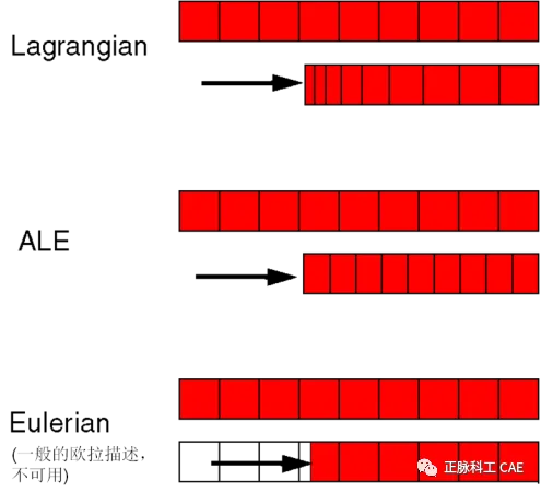 • ALE simulation of axisymmetric forming problems
 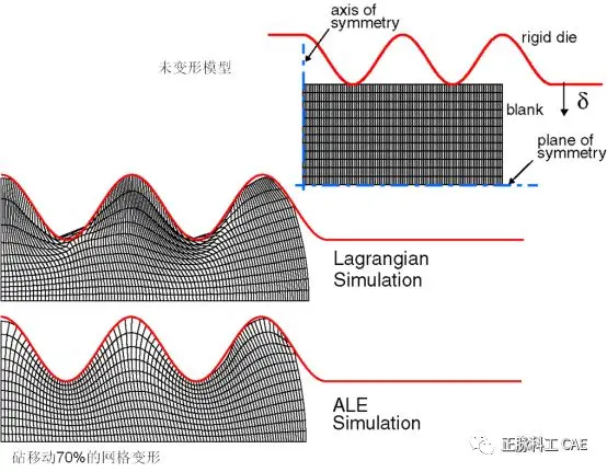 • Using adaptive mesh technology, high-quality meshes can be maintained throughout the analysis process.
 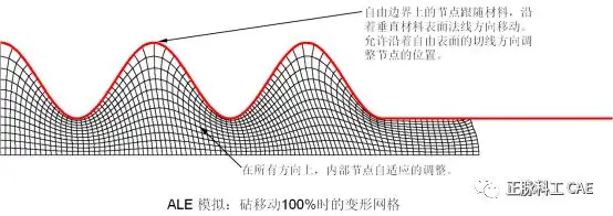 • In transient (Lagrangian-type) problems, such as forging simulations, very little additional input is needed to activate the adaptive mesh function.*HEADING….*ELSET, ELSET=BLANK….*STEP*DYNAMIC, EXPLICIT….*ADAPTIVE MESH, ELSET=BLANK [,FREQUENCY=…,MESH SWEEPS=…]….*END STEP• Adaptive mesh can be used for first-order reduced integration solid elements.• Other element types can exist in the model.Conclusion• Excessively high load rates will produce results with significant inertial effects.• The general recommendation is to limit the rate at which loads are applied, for example, tool speeds should be less than 1% of the material wave speed.• Increasing the load rate from zero in a ramp manner can also improve the accuracy of the quasi-static response.• Use SMOOTH STEP amplitude definition• Mass scaling can be used for rate-dependent material behavior, allowing simulations to be conducted using natural time periods.• Energy balance can be used to evaluate computational results: whether the applied load provides a quasi-static response of the structure.• Since results depend on the speed of the processing (adjusted real or artificial speed through mass scaling), it must be ensured that artificially accelerated processing does not generate unrealistic results.• If confirmation is needed that the results from Abaqus/Explicit are real, the problem can be simplified, and static analysis can be performed using Abaqus/Standard, comparing the analysis results. For comparison purposes, the simplest way to create a simplified test model is to define part of the problem in a two-dimensional manner.• The simplest approach is to establish a two-dimensional computational model of the problem for a trial calculation.• Adaptive mesh technology can maintain high-quality meshes during large deformations.☆ END ☆