
Source: AI Data Research Society


This article is about 2500 words, and it is recommended to read for 7 minutes.
This article introduces node classification.
Source: AI Data Research Society
This article is about 2500 words, and it is recommended to read for 7 minutes.
This article introduces node classification.
1 Naive Node Classification
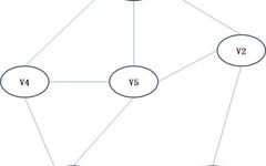
Assuming the network structure is as shown in Figure 1, the vector of the node can be represented as:
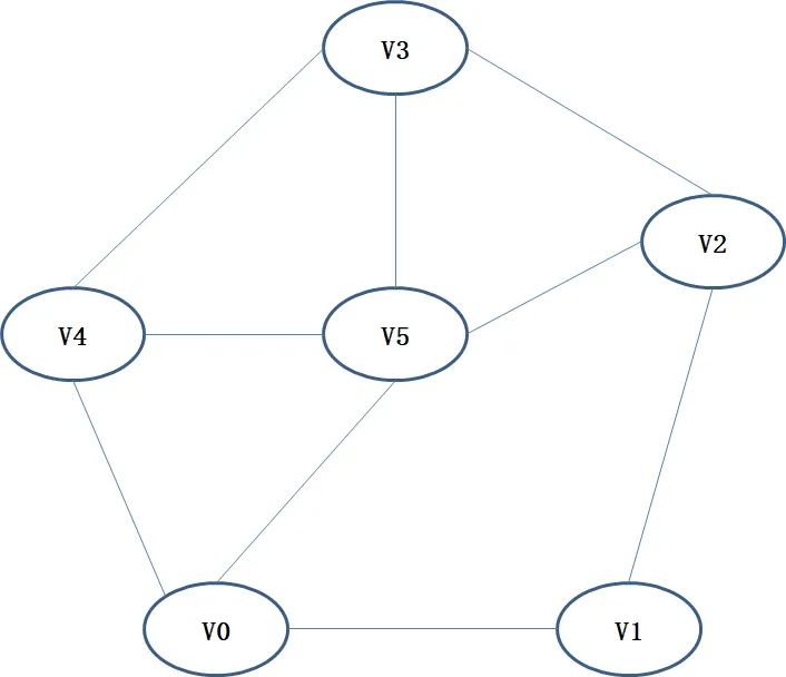
Since the node is connected to , , and , the vector composed of 
will have the vector elements at the positions of , , and taking the value of 1, while the rest take the value of 0. Thus, we obtain conventional structured data, where each element represents a feature of the current node.
[Example] Naive node classification. First, convert the network structure into an adjacency matrix (Adjacency Matrix), and then use a linear kernel SVM model for training.
First, let’s look at the data structure in the network.
import networkx as nx
import numpy as np
import matplotlib.pyplot as plt
from sklearn.model_selection import train_test_split
from sklearn.neighbors import KNeighborsClassifier
from sklearn.svm import SVC
# Data network structure
G = nx.karate_club_graph()
plt.figure(figsize=(15,10))
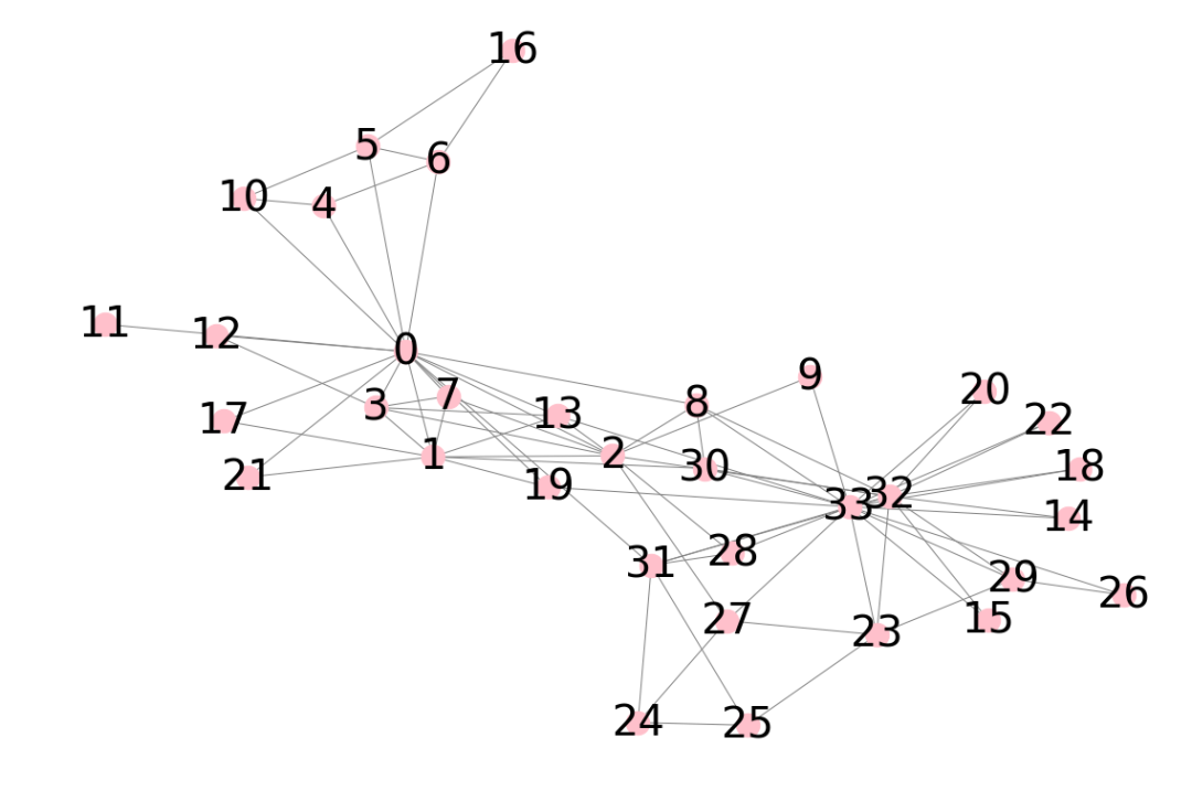
nx.draw( G, with_labels=True, edge_color='grey', node_color='pink', node_size=500, font_size=40, pos=nx.spring_layout(G,k=0.2))
plt.show()The network structure diagram is shown in Figure 2 below:
# Given true labels
groundTruth = [0,0,0,0,0,0,0,0,1,1,0,0,0,0,1,1,0,0,1,0,1,0,1,1,1,1,1,1,0,0,0,0,1,1]
# Define adjacency matrix to convert network nodes into an n X n square matrix
def graphmatrix(G):    n = G.number_of_nodes()    temp = np.zeros([n,n])        for edge in G.edges():        temp[int(edge[0])][int(edge[1])] = 1        temp[int(edge[1])][int(edge[0])] = 1    return temp
edgeMat = graphmatrix(G)
x_train,x_test,y_train,y_test = train_test_split(edgeMat,groundTruth,test_size=0.6,random_state=0)
# Using linear kernel SVM classifier for training
clf = SVC(kernel="linear")
clf.fit(x_train,y_train)
predicted = clf.predict(x_test)
print(predicted)
score = clf.score(x_test,y_test)
print(score)2 Weighted Voting of Neighboring Nodes
Weighted-Vote Relational Neighbor (WVRN) is a typical co-occurring node classification method that does not require a training process. The label of each unlabeled node is obtained through weighted voting from its neighbors:
Where is the label of node . When the labels of the neighboring nodes of node are confirmed, the label of node is also determined. The weights are reflected in the probabilities of the neighboring node labels of node .
[Example] Using the WVRN algorithm for node classification.
Initialize the label values of the samples to 0.5, meaning each sample has a 50% probability of being a positive or negative sample. Use the WVRN algorithm to iterate through the nodes to obtain the final results.
import networkx as nx
import numpy as np
import matplotlib.pyplot as plt
from sklearn.model_selection import train_test_split
from sklearn.metrics import accuracy_score
# Binarization, default 0.5 as threshold, can adjust according to business label distribution
def binary(nodelist,threshold=0.5): for i in range(len(nodelist)): if (nodelist[i]>threshold):nodelist[i]=1.0 else: nodelist[i]=0 return nodelist
G = nx.karate_club_graph() plt.figure(figsize=(15,10))
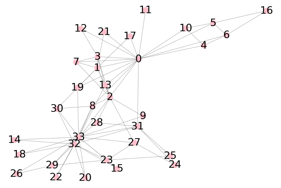
nx.draw( G, with_labels=True, edge_color='grey', node_color='pink', node_size=500, font_size=40, pos=nx.spring_layout(G,k=0.2))
plt.show()The network structure diagram is shown in Figure 3 below:
groundTruth = [0,0,0,0,0,0,0,0,1,1,0,0,0,0,1,1,0,0,1,0,1,0,1,1,1,1,1,1,0,0,0,0,1,1]  max_iter = 10 # Iteration times  nodes = list(G.nodes()) nodes_list = {nodes[i]: i for i in range(0,len(nodes))}
vote = np.zeros(len(nodes))
# x_train, x_test split the labeled and unlabeled nodes, where the values represent node numbers
x_train, x_test, y_train, y_test = train_test_split(nodes,                                        groundTruth, test_size=0.7, random_state=1)

# vote[x_train] assigns true labels, vote[x_test] initializes to 0.5
vote[x_train] = y_train  vote[x_test] = 0.5 # Initialize probability to 0.5
for i in range(max_iter):    # Use only the previous iteration values    last = np.copy(vote)    for u in G.nodes():        if (u in x_train):            continue        temp =0.0        for item in G.neighbors(u):                        # Sum over all neighbors            temp = temp+last[nodes_list[item]]        vote[nodes_list[u]] = temp/len(list(G.neighbors(u)))
# Binarization to obtain classification labels
temp = binary(vote) pred = temp[x_test]
# Calculate accuracy
print(accuracy_score(y_test, pred)) 3 Consistency Label Propagation
[Example] Using the CLPM algorithm for node classification.
import networkx as nx  import numpy as np  from sklearn.model_selection import train_test_split  from sklearn.metrics import accuracy_score  from sklearn import preprocessing  from scipy import sparse
G = nx.karate_club_graph()  groundTruth = [0,0,0,0,0,0,0,0,1,1,0,0,0,0,1,1,0,0,1,0,1,0,1,1,1,1,1,1,0,0,0,0,1,1]
def graphmatrix(G):  # Abstract nodes into edges      n = G.number_of_nodes()      temp = np.zeros([n,n])      for edge in G.edges():          temp[int(edge[0])][int(edge[1])] = 1           temp[int(edge[1])][int(edge[0])] = 1      return temp
def propagation_matrix(G):      # Matrix normalization      degrees = G.sum(axis=0)      degrees[degrees==0] += 1  # Avoid division by zero      D2 = np.identity(G.shape[0])      for i in range(G.shape[0]):          D2[i,i] = np.sqrt(1.0/degrees[i])      S = D2.dot(G).dot(D2)      return S  # Define function to take the maximum value   def vec2label(Y):      return np.argmax(Y,axis=1)
edgematrix = graphmatrix(G)  S = propagation_matrix(edgematrix)
Ap = 0.8  cn = 2  max_iter = 10
# Define iteration function  F = np.zeros([G.number_of_nodes(),2])  X_train, X_test, y_train, y_test = train_test_split(list(G.nodes()),                                        groundTruth, test_size=0.7, random_state=1)for (node, label) in zip(X_train, y_train):      F[node][label] = 1
Y = F.copy()
for i in range(max_iter):      F_old = np.copy(F)      F = Ap*np.dot(S, F_old) + (1-Ap)*Y
temp = vec2label(F)  pred = temp[X_test]  print(accuracy_score(y_test, pred))
The running result is 0.75, indicating that the current model’s prediction accuracy is 0.75.