Click the “CVer” above to add it to your “Favorites” list.
Essential insights delivered promptly.
This article is reprinted from: Smarter
Since the introduction of the Transformer, it has dominated the NLP field. However, its impact in the CV domain has been moderate, with initial thoughts suggesting it was unsuitable for CV until recently. A few Transformer papers in the computer vision field have emerged, showing performance that rivals the SOTA of CNNs, providing new imaginative space for computer vision.
This article does not focus on the principles and detailed implementations of Transformers (many high-quality analytical articles on Transformers can be found on Zhihu for those interested), but rather on the innovations Transformers bring to the computer vision field.
First, we will briefly review Transformer, followed by an introduction to several recent Transformer papers in the computer vision field, including ViT for image classification, DETR, and Deformable DETR for object detection. From these papers, we can see that the paradigm of Transformer in computer vision is taking shape, roughly summarized as: Embedding->Transformer->Head.
Some interesting points are written at the end~~
01
Transformer
Transformer Explained: http://jalammar.github.io/illustrated-transformer/
Below, we will briefly introduce the Transformer structure using machine translation as an example.
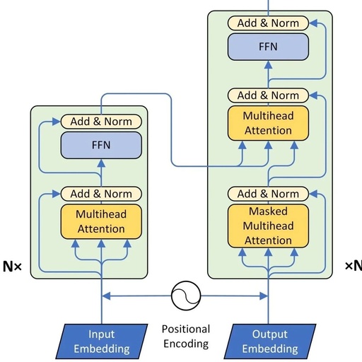
1. Encoder-Decoder
The Transformer structure can be represented as two parts: Encoder and Decoder.
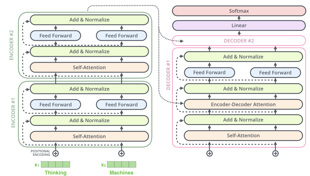
Encoder and Decoder are primarily composed of Self-Attention and Feed-Forward Network components. Self-Attention consists of Scaled Dot-Product Attention and Multi-Head Attention components.
The formula for Scaled Dot-Product Attention is:
Multi-Head Attention formula:
The Feed-Forward Network formula is:
2. Positional Encoding
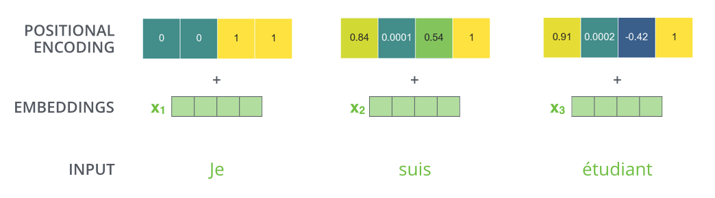
As shown in the figure, since the machine translation task is related to the order of input words, the Transformer introduces positional encoding when encoding the embedding vectors of input words, allowing the Transformer to distinguish the positions of input words.
The formula for introducing positional encoding is:
is the position, is the dimension, and is the dimension of the input word’s embedding vector.
3. Self-Attention
3.1 Scaled Dot-Product Attention
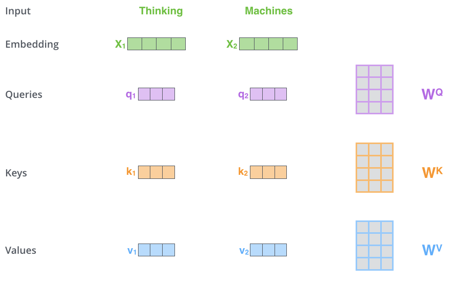
In Scaled Dot-Product Attention, the embedding vector of each input word is transformed into Query vector ( ), Key vector ( ), and Value vector ( ) through three matrices , and respectively.
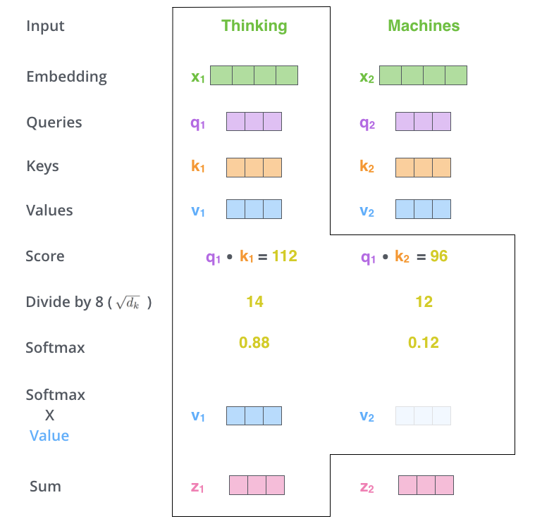
As shown in the figure, the computation process of Scaled Dot-Product Attention can be divided into seven steps:
-
Each input word is converted into an embedding vector.
-
According to the embedding vector, obtain the , , three vectors.
-
Calculate using , vectors: .
-
Normalize by dividing by .
-
Use the activation function to calculate .
-
multiply the Value to get the score for each input vector .
-
The sum of all input vector scores is: .
The matrix form of the above steps can be expressed as:
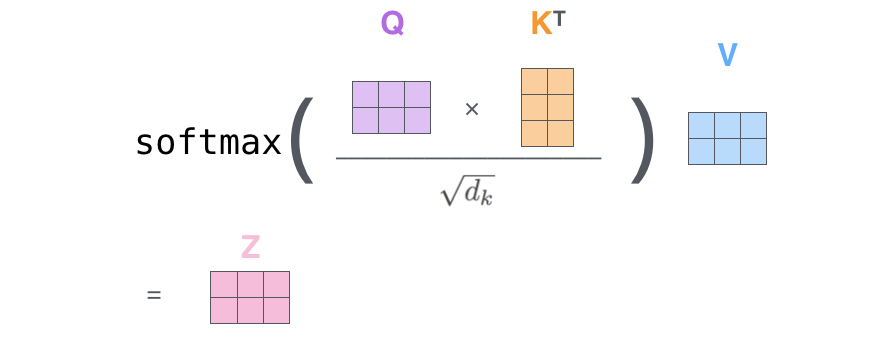
This is consistent with the Scaled Dot-Product Attention formula.
3.2 Multi-Head Attention
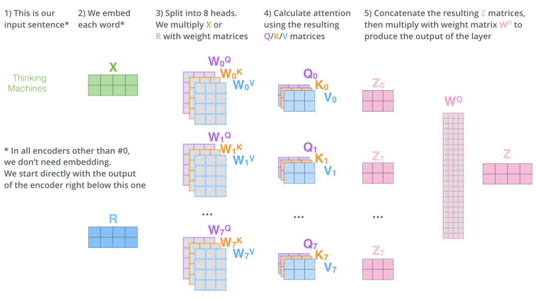
As shown in the figure, Multi-Head Attention is an ensemble of h different Scaled Dot-Product Attention. For example, with h=8, the steps of Multi-Head Attention are as follows:
-
Input data into 8 different Scaled Dot-Product Attention, obtaining 8 weighted feature matrices .
-
Stack the 8 into a large feature matrix by columns.
-
The feature matrix passes through a fully connected layer to obtain output .
Both Scaled Dot-Product Attention and Multi-Head Attention include a shortcut mechanism.
02
ViT
ViT cleverly applies the Transformer to the image classification task, achieving performance comparable to SOTA with less computational load.

The Vision Transformer (ViT) splits the input image into 16×16 patches, performs a linear transformation to reduce dimensions while embedding positional information, and then sends it into the Transformer, avoiding pixel-level attention computations. Similar to the [class] token in BERT, ViT adds an extra learnable [class] token to the input sequence of the Transformer, with the output of this position in the Transformer Encoder serving as the image feature.
Where is the original image resolution, is the resolution of each image patch. is the length of the Transformer input sequence.
ViT discards the inductive bias issue of CNNs, making it more conducive to learning knowledge on large-scale datasets, achieving near SOTA in many image classification tasks.
03
DETR
DETR uses a set loss function as a supervision signal for end-to-end training, predicting all objects simultaneously. The set loss function uses a bipartite matching algorithm to match predicted objects with ground truth. It treats the object detection task as a set prediction problem, simplifying the training process and avoiding complex processing like anchors and NMS.
DETR mainly consists of two parts: architecture and set prediction loss.
1. Architecture
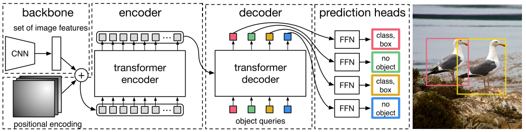
DETR first uses CNN to embed the input image into a two-dimensional representation, then transforms this two-dimensional representation into a one-dimensional representation and combines it with positional encoding to input into the encoder. The decoder takes a small fixed number of learned object queries (which can be understood as positional embeddings) and the encoder’s output as input. Finally, each output embedding from the decoder is passed to a shared feed-forward network (FFN), which can predict a detection result (including class and bounding box) or a “no object” class.
1.1 Transformer
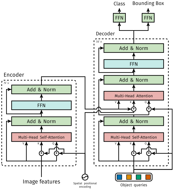
1.1.1 Encoder
The feature map output from the Backbone is converted into a one-dimensional representation, obtaining the feature map, which is then combined with positional encoding as the input to the Encoder. Each Encoder consists of Multi-Head Self-Attention and FFN.
Unlike the Transformer Encoder, since the Encoder has position invariance, DETR adds positional encoding to each Multi-Head Self-Attention to ensure the position sensitivity of object detection.
1.1.2 Decoder
Since the Decoder also has position invariance, the object queries (which can be understood as positional embeddings for learning different objects) must be different to produce different results, and they are added to each Multi-Head Attention. The object queries are transformed into an output embedding by the Decoder, and then the output embedding independently decodes the predicted results, including boxes and classes. By using both Self-Attention and Encoder-Decoder Attention on the input embeddings, the model can utilize the relationships between objects for global reasoning.
Unlike the Transformer Decoder, each Decoder in DETR outputs objects in parallel, while the Transformer Decoder uses an autoregressive model to output objects serially, predicting one element of the output sequence at a time.
1.1.3 FFN
The FFN consists of 3 layers of perceptrons and one layer of linear projection. The FFN predicts the normalized center coordinates, length, width, and class of the box.
DETR predicts a fixed number of boxes, and is usually much larger than the actual number of objects, so an additional empty class is used to indicate that the predicted box does not contain an object.
2. Set prediction loss
The main difficulty in training the DETR model is how to measure the predicted results (class, location, quantity) against the ground truth. The loss function proposed by DETR can produce optimal bipartite matching between predictions and ground truth (establishing a one-to-one relationship between predictions and ground truth), and then optimize the loss.
Let y represent the set of ground truth, and let represent the set of predicted results. Assuming is greater than the number of objects in the image, it can be considered as a set of size filled with empty classes (no objects). The search for different permutations of the two sets of elements aims to minimize the loss, and the optimal arrangement that minimizes the loss corresponds to the maximum matching in the bipartite graph, as follows:
Where represents the matching loss of predictions and ground truth for the element. The bipartite matching is obtained using the Hungarian algorithm.
The matching loss simultaneously considers the accuracy of the predicted class and predicted box. Each element of the ground truth can be regarded as , where represents the class label (which can be an empty class) and represents the ground truth box, and the elements specified by the bipartite matching for the predicted class are represented as , and the predicted box as .
The first step is to find a one-to-one matching between predictions and ground truth, and the second step is to calculate the Hungarian loss.
The formula for the Hungarian loss is as follows:
Where combines L1 loss and generalized IoU loss, as follows:
The experiments and visual analysis of the ViT and DETR papers are very enlightening; those interested can take a closer look~~
04
Deformable DETR
From DETR, it’s still not enough to catch up with CNNs due to long training times. The emergence of Deformable DETR has given me new expectations for Transformers.
Deformable DETR replaces the attention mechanism in DETR with Deformable Attention, making the DETR paradigm detector more efficient, accelerating convergence speed by 10 times.
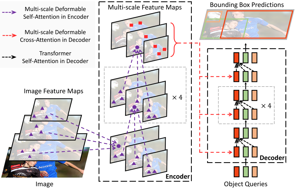
The Deformable Attention proposed by Deformable DETR can alleviate the slow convergence speed and high complexity of DETR. It combines the sparse spatial sampling capability of deformable convolution with the relational modeling capability of transformers. Deformable Attention can consider a small set of sampling locations as a pre-filter to highlight the key features of all feature maps and can naturally extend to fuse multi-scale features. Multi-scale Deformable Attention itself can exchange information between multi-scale feature maps without the need for FPN operations.
1. Deformable Attention Module
Given a query element (such as the target word in the output sentence) and a set of key elements (such as the source words in the input sentence), Multi-Head Attention can adaptively aggregate the information of keys based on the relevance of query-key pairs. To allow the model to focus on information from different representation subspaces and different locations, the multi-head information is aggregated with weights. Where represents the query element (feature represented as ), represents the key elements (features represented as ), is the feature dimension, and and are the sets of and .
The Multi-Head Attention formula for the Transformer is expressed as:
Where specifies the attention head, and are learnable parameters, and the attention weights are normalized, where is a learnable parameter. To distinguish different spatial positions, and typically introduce positional embedding.
For the Transformer Encoder in DETR, both query and key elements are pixels in the feature map.
The Multi-Head Attention formula for DETR is expressed as:
Where .
DETR has two main issues: it requires more training time to converge and performs relatively poorly on small object detection. Essentially, this is because the Multi-Head Attention of the Transformer computes attention across all spatial locations of the input image, while Deformable DETR’s Deformable Attention focuses only on a small number of key sampling points around reference points, which can alleviate convergence issues and input resolution limitations.
Given an input feature map , is represented as the query element (feature represented as), and the two-dimensional reference points are represented as . The Deformable Attention formula for Deformable DETR is expressed as:
Where specifies the attention head, specifies the sampled keys, and represents the total number of sampled keys ( ). and represent the sampling offset and attention weights for the sampling point in the attention head. The attention weights are in the range of [0,1], normalized as . is represented as a two-dimensional real number without constraints. Since is a score, bilinear interpolation must be used for calculation.
2. Multi-scale Deformable Attention Module
Deformable Attention can naturally extend to multi-scale feature maps. is represented as the input multi-scale feature maps, . represents the normalized coordinates of the reference point for each query element . The Multi-scale Deformable Attention formula for Deformable DETR is expressed as:
Where specifies the attention head, specifies the input feature layer, specifies the sampled keys, and represents the total number of sampled keys ( ). and represent the sampling offset and attention weights for the sampling point in the feature layer’s attention head. The attention weights are in the range of [0,1], normalized as .
3. Deformable Transformer Encoder
Replace all attention in DETR with multi-scale deformable attention. The input and output of the encoder are multi-scale feature maps with the same resolution. The encoder extracts multi-scale feature maps from ResNet (obtained by 3×3 stride 2 convolution).
Using multi-scale deformable attention in the encoder, the output is multi-scale feature maps with the same resolution as the input. Both query and key come from the pixels of the multi-scale feature maps. For each query pixel, the reference point is itself. To determine which feature layer the query pixel comes from, in addition to positional embedding, a scale-level embedding is added. Unlike the fixed encoding of positional embedding, scale-level embedding is randomly initialized and learned through training.
4. Deformable Transformer Decoder
In the decoder, there are both cross-attention and self-attention. The query elements for these two types of attention are the object queries. In cross-attention, object queries extract features from feature maps, while the key elements are the feature maps output from the encoder. In self-attention, the object queries interact with each other, and the key elements are also the object queries. Since Deformable Attention is used for feature extraction of key elements from feature maps, in the decoder, deformable attention only replaces cross-attention.
Because multi-scale deformable attention extracts image features around reference points, it allows the detection head to predict the offsets of boxes relative to the reference points, further reducing optimization difficulty.
05
Complexity Analysis
Assuming the number of queries and keys is , ( ), and the dimension is , with the number of key sampling points as and the size of the image’s feature map as , and the kernel size as .
Convolution Complexity
-
To ensure the input and output are the same in the first dimension, padding must be applied to the input, as the kernel size is (the actual shape of the kernel is ).
-
The computational complexity of a convolution kernel of size is , and it is performed times, thus the complexity is .
-
To ensure the third dimension is equal, convolution kernels are needed, so the time complexity of the convolution operation is .
Self-Attention Complexity
-
has a computational complexity of .
-
Similarity Calculation : with operation, resulting in matrix, complexity is .
-
Calculation: For each row, it involves , complexity is , thus the complexity for n rows is .
-
Weighted Sum: with operation, resulting in matrix, complexity is .
-
Thus, the final time complexity of Self-Attention is .
Transformer
The complexity of Self-Attention is .
ViT
The complexity of Self-Attention is .
DETR
The complexity of Self-Attention is .
Deformable DETR
The complexity of Self-Attention is .
For detailed analysis, refer to the original papers.
06
Several Questions
How to understand? Why not use the same and ?
1. From the physical meaning of dot product, the dot product of two vectors represents the similarity between the two vectors.
2. ‘s physical meaning is the same, both represent the matrix composed of different tokens in the same sentence. Each row in the matrix represents a token’s word embedding vector. Suppose a sentence “Hello, how are you?” has a length of 6 and an embedding dimension of 300, then both are matrices of (6,300).
Therefore, the dot product of and can be understood as calculating the similarity of each token in a sentence with other tokens in the same sentence. This similarity can be understood as the attention score, which indicates the degree of focus. Although the attention score matrix is obtained, this matrix is derived from various calculations and is already difficult to represent the original sentence, while still represents the original sentence. Thus, the attention score matrix can be multiplied by to yield a weighted result.
Through the above explanation, we know that the dot product of and is to obtain an attention score matrix to refine . Using different and to calculate can be understood as projecting in different spaces. It is precisely because of this projection in different spaces that the expressive power is increased, making the attention score matrix obtained have higher generalization capability. Here, I explain my understanding of generalization capability; since and use different , the resulting matrices are completely different, thus enhancing the expressive power. However, if we don’t use and directly use and , the attention score matrix will be a symmetric matrix, leading to poor generalization capability, and the refining effect on will deteriorate.
For detailed analysis, refer to the linked articles.
https://medium.com/dissecting-bert/dissecting-bert-part-1-d3c3d495cdb3
https://www.zhihu.com/question/319339652/answer/730848834
How to improve Position Embedding?
This remains an open question, and there are some high-quality discussions on Zhihu. For detailed analysis, refer to the linked articles.
NLP: https://www.zhihu.com/question/347678607/answer/864217252
CV: https://zhuanlan.zhihu.com/p/99766566
Why does ViT add a [CLS] token? Why is the vector corresponding to the [CLS] token used as the semantic representation of the entire sequence?
Similar to BERT, ViT adds a learnable [CLS] token at the beginning of the sequence. For example, in BERT, a [CLS] token is added before the first sentence, and the vector corresponding to this token in the last layer can serve as the semantic representation of the entire sentence for downstream classification tasks, etc.
The vector corresponding to the [CLS] token is used as the semantic representation of the entire text because, compared to other words already present in the text, this symbol, which has no obvious semantic information, can more “fairly” merge the semantic information of various words in the text, thus better representing the semantics of the entire sentence.
What is inductive bias?
Inductive bias is a subtle concept in machine learning: many learning algorithms often make certain assumptions about the learning problem, and these assumptions are called inductive bias. Inductive bias can be understood as inferring certain rules (heuristics) from observed phenomena in real life and then constraining the model, which can serve as a “model selection” role, selecting models that better conform to real-world rules from the hypothesis space. Inductive bias can be understood as the “prior” in Bayesian learning.
Inductive bias is also used in deep learning. In CNNs, it is assumed that features have locality, meaning that merging adjacent features will more easily yield a solution; in RNNs, it is assumed that each computation at a moment depends on historical computations; and the attention mechanism is also a rule inferred from human intuition and life experience.
Transformers can avoid the locality inductive bias problem present in CNNs. For instance, in DETR, an experiment was conducted where synthetic images were created to validate DETR’s generalization ability, demonstrating that DETR can completely identify all 24 giraffes in the synthetic image, despite the training set not containing images with more than 13 giraffes. This confirms that DETR avoids the inductive bias problem of CNNs.
https://www.zhihu.com/question/264264203/answer/830077823
Bipartite matching? Hungarian algorithm?
Given a bipartite graph G, a subgraph M of G is called a matching if no two edges in the edge set {E} of M are incident to the same vertex. The maximum matching of a bipartite graph can be obtained using the Hungarian algorithm.
For detailed analysis, refer to the linked articles.
https://liam.page/2016/04/03/Hungarian-algorithm-in-the-maximum-matching-problem-of-bigraph/
https://zhuanlan.zhihu.com/p/62981901
What is the relationship between the positional embedding, object queries, and slots in DETR?
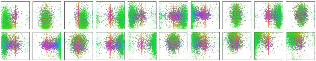
DETR visualizes the 20 slots predicted by the decoder. It can be observed that each slot learns the scale size of a specific area. From this perspective, object queries are somewhat similar to the anchors in object detectors like Faster-RCNN, where the positional embedding information from the encoder helps each slot look for targets in the specific areas it has learned.
What are the advantages and disadvantages of Transformer compared to CNN?
Advantages:
Transformers focus on global information, capable of modeling longer-distance dependencies, while CNNs focus on local information, having weaker abilities to capture global information.
Transformers avoid the inductive bias problem present in CNNs.
Disadvantages:
Transformers have higher complexity than CNNs, but ViT and Deformable DETR provide solutions to reduce the complexity of Transformers.
07
Summary
Transformers have brought significant innovations to image classification and object detection, and segmentation, tracking, and video tasks are not far behind.
The relationship between NLP and CV is becoming increasingly interesting. Although there is much controversy, just imagine, if NLP and CV could express themselves using a single paradigm, how terrifying would that be? In the future, could images and text be freely converted? Is strong artificial intelligence capable of perception and reasoning not far away? (Just a thought)
Moving towards the unification of NLP and CV.
Reference
[1] Attention Is All You Need
[2] An Image is Worth 16*16 Words: Transformers for Image Recognition at Scale
[3] End-to-End Object Detection with Transformers
[4] Deformable DETR: Deformable Transformers for End-to-End Object Detection
Download 1: Dive into Deep Learning
Reply in the CVer public account backend with:Dive into Deep Learning to download547 pages of the electronic book and source code. This book is a deep learning textbook designed for Chinese readers, combining text, formulas, images, code, and running results. It comprehensively covers deep learning from model construction to model training, as well as their applications in computer vision and natural language processing.

Download 2: CVPR / ECCV 2020 Open Source Code
Reply in the CVer public account backend with:CVPR2020, to download the collection of open-source papers from CVPR 2020
Reply in the CVer public account backend with:ECCV2020, to download the collection of open-source papers from ECCV 2020
Important! CVer-Paper Writing and Submission Communication Group Established
Scan to add CVer assistant, to apply to join CVer-Paper Writing and Submission WeChat communication group, which currently has over 2300 members, aiming to discuss top conferences (CVPR/ICCV/ECCV/NIPS/ICML/ICLR/AAAI, etc.), top journals (IJCV/TPAMI/TIP, etc.), SCI, EI, Chinese core, and other writing and submission matters.
At the same time, you can also apply to join the CVer large group and subdivided technical groups, covering:Object detection, image segmentation, object tracking, face detection & recognition, OCR, pose estimation, super-resolution, SLAM, medical imaging, Re-ID, GAN, NAS, depth estimation, autonomous driving, reinforcement learning, lane line detection, model pruning & compression, denoising, dehazing, deraining, style transfer, remote sensing images, behavior recognition, video understanding, image fusion, paper submission & communication, PyTorch and TensorFlow and other groups.
Be sure to note:Research Direction + Location + School/Company + Nickname (e.g.,Paper Writing + Shanghai + SJTU + Kaka), based on the format noted, can be approved faster and invited into the group.