

This article introduces how the diffusion model works.
The rise of diffusion models can be seen as a major factor in the recent breakthroughs in the field of AI-generated art. The development of the stable diffusion model allows us to easily create wonderful artistic illustrations through a text prompt. So in this article, I will explain how they work.
Diffusion Model
The training of diffusion models can be divided into two parts:
-
Forward diffusion → adding noise to the image.
-
Reverse diffusion process → removing noise from the image.
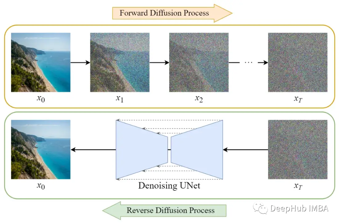
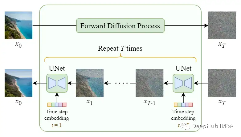
Forward Diffusion Process
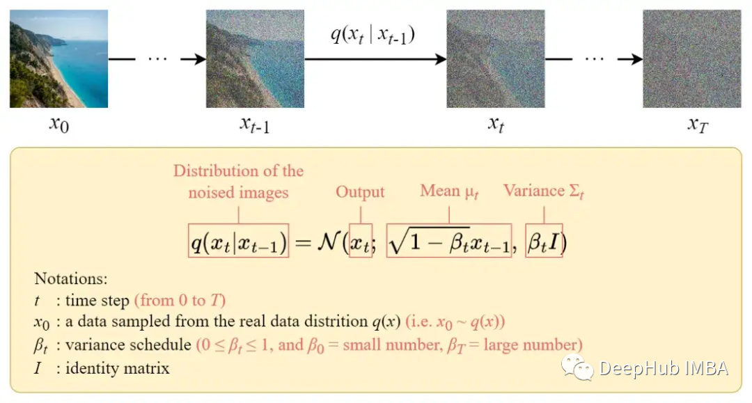
The forward diffusion process gradually adds Gaussian noise to the input image x₀ over T steps. This process will produce a series of noisy image samples x₁, …, x_T.
As T → ∞, the final result will become a completely noisy image, just like sampling from an isotropic Gaussian distribution.
However, we can use a closed-form formula to sample directly from the noisy image at a specific time step t, instead of designing an algorithm to iteratively add noise to the image.
Closed-Form Formula
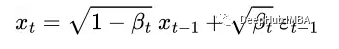
The closed-form sampling formula can be derived using the reparameterization trick.
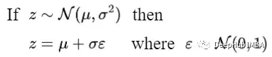
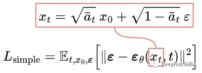
Using this trick, we can express the sampled image xₜ as:
We can then recursively expand it, ultimately obtaining the closed-form formula:
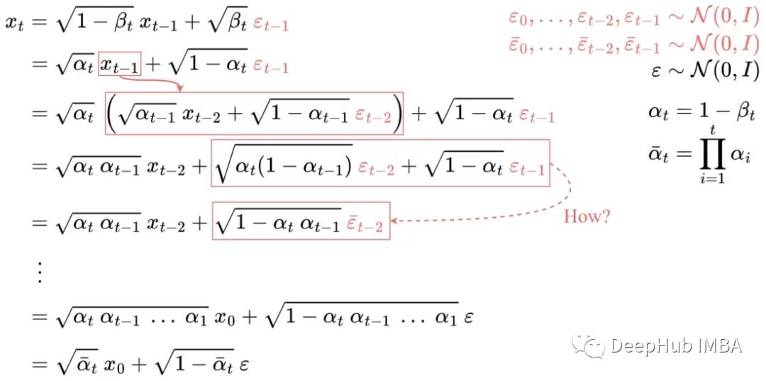
Here, ε is an i.i.d. (independent and identically distributed) standard normal random variable. It is important to distinguish them using different symbols and subscripts, as they are independent and their values may differ after sampling.
But how did the above formula jump from line 4 to line 5?
Some people find this step hard to understand. Below I will detail how it works:

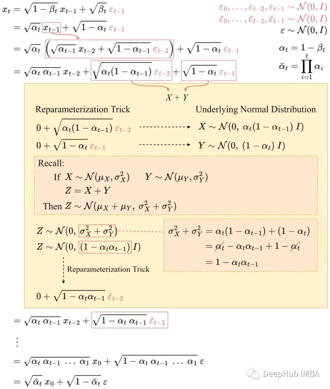
Let’s denote these two terms as X and Y. They can be viewed as samples from two different normal distributions, i.e., X ~ N(0, αₜ(1-αₜ₋₁)I) and Y ~ N(0, (1-αₜ)I).
The sum of two independent normal random variables is also normally distributed. That is, if Z = X + Y, then Z ~ N(0, σ²ₓ+σ²ᵧ). Therefore, we can combine them and reparameterize the merged normal distribution.
Repeating these steps will yield a formula that is only related to the input image x₀:
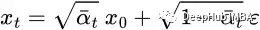
Now we can use this formula to sample xₜ directly at any time step, making the forward process faster.
Reverse Diffusion Process
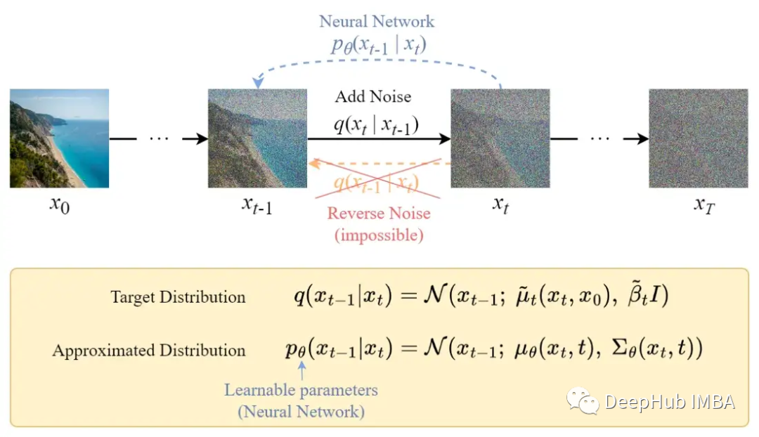
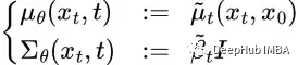
Unlike the forward process, we cannot use q(xₜ₋₁|xₜ) to reverse the noise because it is difficult to handle (non-computable). Therefore, we need to train a neural network pθ(xₜ₋₁|xₜ) to approximate q(xₜ₋₁|xₜ). The approximation pθ(xₜ₋₁|xₜ) follows a normal distribution, with the mean and variance set as follows:
Loss Function
The loss is defined as the negative log-likelihood:
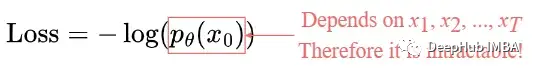
This setup is very similar to that in VAEs. We can optimize the variational lower bound instead of optimizing the loss function itself.
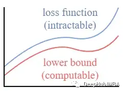
By optimizing a computable lower bound, we can indirectly optimize the intractable loss function.
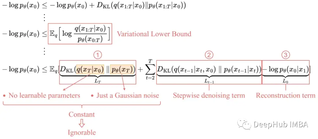
Through expansion, we find that it can be represented by the following three terms:
1. L_T: Constant term
Since q has no learnable parameters, p is just a Gaussian noise probability, this term will be a constant during training and can be ignored.
2. Lₜ₋₁: Stepwise denoising term
This term compares the target denoising step q and the approximate denoising step pθ. By conditioning on x₀, q(xₜ₋₁|xₜ, x₀) becomes easy to handle.
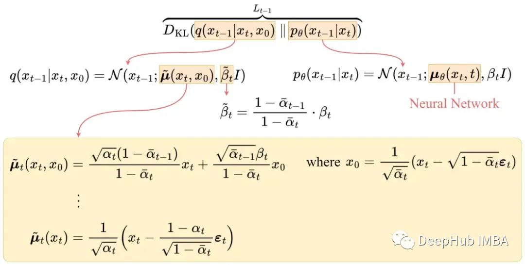
After a series of derivations, the above figure shows the average value μ′ₜ of q(xₜ₋₁|xₜ,x₀). To approximate the target denoising step q, we only need to use the neural network to approximate its mean. So we set the approximate mean μθ to have the same form as the target mean μ̃ₜ (using a learnable neural network εθ):
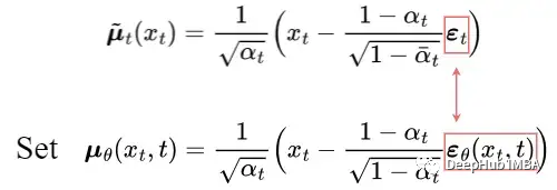
The comparison between the target mean and the approximation can be performed using Mean Squared Error (MSE):
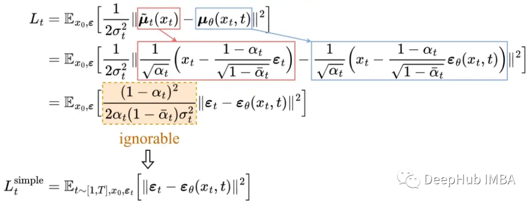
Through experimentation, it was found that by ignoring the weighted term and simply comparing the target noise and predicted noise with MSE, better results can be obtained. Therefore, to approximate the required denoising step q, we only need to use the neural network εθ to approximate the noise εₜ.
3. L₀: Reconstruction term
This is the reconstruction loss of the final denoising step, which can be ignored during training because:
-
The same neural network used in Lₜ₋₁ can approximate it.
-
Ignoring it will improve sample quality and make implementation easier.
So the final simplified training objective is as follows:
We find that training our model on the true variational boundary yields better code length than training on the simplified objective, as expected, but the latter yields the best sample quality.[2]
Through testing, training the model on the variational boundary reduces the code length compared to training on the simplified objective, but the latter produces the best sample quality.[2]
U-Net Model
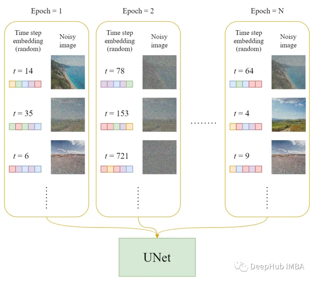
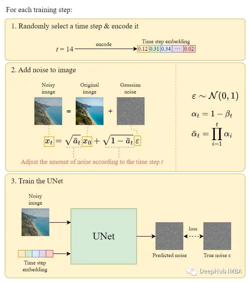
In each training iteration
-
A random time step t is selected for each training sample (image).
-
Gaussian noise is applied to each image (corresponding to t).
-
The time step is transformed into an embedding (vector).
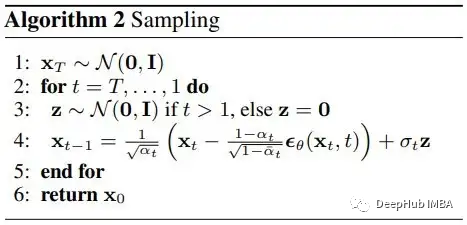
Pseudocode for the training process
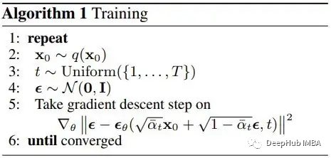
The official training algorithm is shown above, and the following figure illustrates how the training steps work:
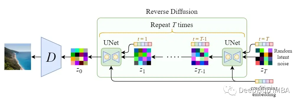
Reverse diffusion
We can use the above algorithm to generate images from noise. The chart below illustrates this:
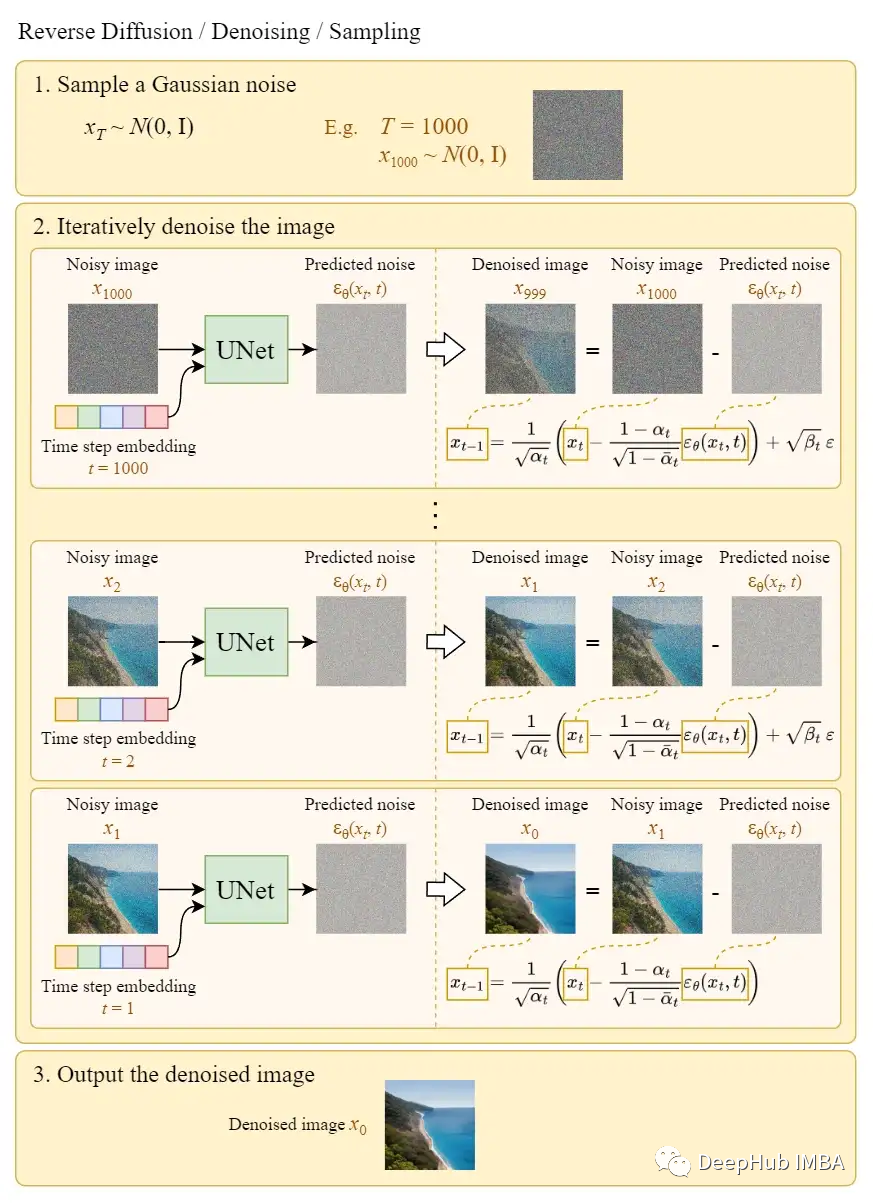
In the final step, simply output the learned mean μθ(x₁,1) without adding noise. Reverse diffusion is what we call the sampling process, which is the process of drawing images from Gaussian noise.
Speed Issues of Diffusion Models
The diffusion (sampling) process iteratively provides full-sized images to U-Net to obtain the final result. This makes pure diffusion models extremely slow when the total number of diffusion steps T and the image size are large.
Stable diffusion was designed to solve this problem.
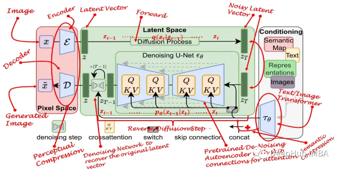
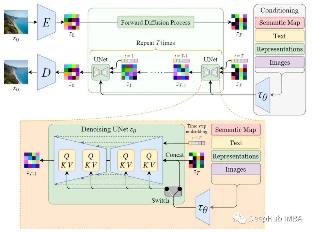
Stable Diffusion
The original name of the stable diffusion model is Latent Diffusion Model (LDM). As its name suggests, the diffusion process occurs in the latent space. This is why it is much faster than pure diffusion models.
Latent Space
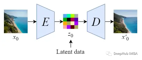
First, train an autoencoder to learn to compress image data into low-dimensional representations.
Using the trained encoder E, full-sized images can be encoded into low-dimensional latent data (compressed data). Then, using the trained decoder D, the latent data can be decoded back into images.
Diffusion in Latent Space
After encoding the images, the forward and reverse diffusion processes are performed in the latent space.
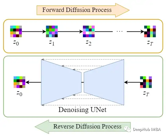
-
Forward diffusion process → adding noise to the latent data
-
Reverse diffusion process → removing noise from the latent data
Conditional Effects/Modulation
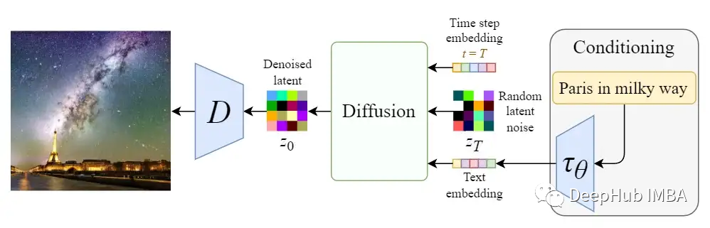
The real power of the stable diffusion model lies in its ability to generate images from text prompts. This is achieved by modifying the internal diffusion model to accept conditional inputs.
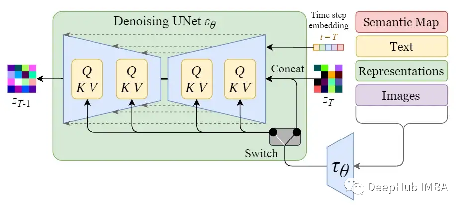
By enhancing its denoising U-Net with a cross-attention mechanism, the internal diffusion model is transformed into a conditional image generator.
The switch in the above figure is used to control between different types of modulation inputs:
-
For text inputs, language models 𝜏θ (e.g., BERT, CLIP) are first used to convert them into embeddings (vectors), which are then mapped to U-Net layers via (multi-head) Attention(Q, K, V).
-
For other spatially aligned inputs (e.g., semantic mappings, images, repairs), concatenation can be used to complete the modulation.
Training
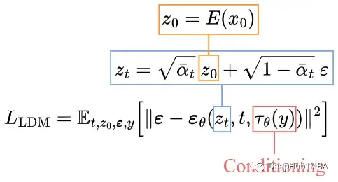
The training objective (loss function) is very similar to that in pure diffusion models. The only changes are:
-
Input latent data zₜ instead of image xₜ.
-
U-Net adds conditional input 𝜏θ(y).
Sampling
Since the size of the latent data is much smaller than that of the original image, the denoising process is much faster.
Comparison of Architectures
A comparison of the overall architectures of pure diffusion models and stable diffusion models (latent diffusion models).
Diffusion Model
Stable Diffusion (Latent Diffusion Model)
To summarize quickly:
-
Diffusion models are divided into forward diffusion and reverse diffusion.
-
Forward diffusion can be computed using a closed-form formula.
-
Reverse diffusion can be accomplished using a trained neural network.
-
To approximate the required denoising step q, we only need to use the neural network εθ to approximate the noise εₜ.
-
Training on the simplified loss function yields better sample quality.
-
Stable diffusion (latent diffusion model) performs the diffusion process in latent space, thus being much faster than pure diffusion models.
-
The pure diffusion model was modified to accept conditional inputs, such as text, images, semantics, etc.
Citations
Editor: Wang Jing
Proofreader: Lin Yilin