How to Deceive Neural Networks to Recognize Pandas as Vultures

Authorized Reprint from CSDN

Source: codewords.recurse.com

Translator: Liu Diwei, Reviewer: Liu Xiangyu, Editor: Zhong Ha

Website: http://www.csdn.net

Abstract: This article is based on the author’s reading of papers and practical tests, attempting to deceive neural networks. It gradually analyzes neural networks and the mathematical principles behind them, from tool installation to model training. The article also provides downloadable demonstration code.

Magical Neural Networks

When I open Google Photos and search for “skyline,” it finds this photo of the New York skyline that I took in August, even though I hadn’t tagged it before.

When I search for ‘cathedral,’ Google’s neural network finds the cathedrals and churches I have seen. This seems magical.

Of course, neural networks are not magical at all! Recently, I read a paper titled “Explaining and Harnessing Adversarial Examples,” which further diminished my sense of mystery about neural networks.

This paper explains how to deceive neural networks into making astonishing mistakes by leveraging simpler (more linear!) facts about the network than you might imagine. We will use a linear function to approximate this network!

The key is to understand that this does not explain all (or most) types of errors made by neural networks! There are many possible mistakes! But it does provide us with some inspiration regarding specific types of errors, which is great.

Before reading this paper, I had the following three understandings of neural networks:

• They perform excellently in image classification (when I search for “baby,” it finds pictures of my friend’s cute child)

• Everyone online is talking about “deep” neural networks

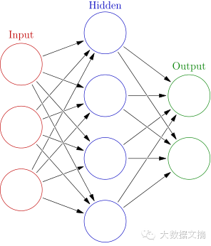
• They consist of multiple layers of simple functions (usually sigmoid), structured as shown in the figure below:

Errors

My fourth (and final) understanding of neural networks is that they sometimes make ridiculous mistakes. Spoiler alert for the results later in this article: these are two images, and the article will show how the neural network classifies them. We can make it believe that the black image below is a paper towel, while the panda will be recognized as a vulture!

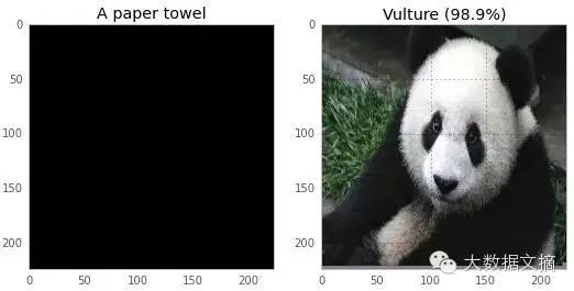
Now, this result does not surprise me because machine learning is my job, and I know that machine learning tends to produce strange results. But to solve this super strange error, we need to understand the principles behind it! We will learn some knowledge related to neural networks, and then I will teach you how to make the neural network think that a panda is a vulture.

Making the First Prediction

We first load a neural network, make some predictions, and then break those predictions. This sounds great. But first, I need to get a neural network on my computer.

I installed Caffe on my computer, a neural network software developed by contributors from the Berkeley Vision and Learning Center (BVLC) community. I chose it because it was the first software I could find, and I could download a pre-trained network. You can also try Theano or TensorFlow. Caffe has very clear installation instructions, which means I only needed to spend 6 hours familiarizing myself before officially using it for work.

If you want to install Caffe, you can refer to the program I wrote, which will save you more time. Just go to the neural-networks-are-weird repo and follow the instructions to run it. Warning: it will download about 1.5G of data and require compiling a lot of things. Below are the commands to build it (only 3 lines!), and you can also find them in the README file under the repository.

git clone https://github.com/jvns/neural-nets-are-weird
cd neural-nets-are-weird
docker build -t neural-nets-fun:caffe .
docker run -i -p 9990:8888 -v $PWD:/neural-nets -t neural-nets-fun:caffe /bin/bash -c 'export PYTHONPATH=/opt/caffe/python && cd /neural-nets && ipython notebook --no-browser --ip 0.0.0.0'

This will start the IPython notebook service on your computer, and then you can use Python to make neural network predictions. It needs to run on the local port 9990. If you don’t want to do it this way, that’s totally fine. I have also included the experimental images in this article.

Once we have the IPython notebook up and running, we can start running the code and making predictions! Here, I will paste some nice pictures and a few code snippets, but the complete code and detailed details can be found here.

We will use a neural network called GoogLeNet, which won several competitions in LSVRC 2014. Correct classification is among the top 5 guesses of the network, consuming 94% of the time. This is the network from the paper I read. (If you want a good read, you can check out the article that humans can’t do better than GoogLeNet. Neural networks are truly magical.)

First, let’s classify an adorable kitten using the network:

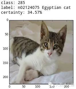
Below is the code for classifying the kitten:

image = '/tmp/kitten.png'
# preprocess the kitten and resize it to 224x224 pixels
net.blobs['data'].data[...] = transformer.preprocess('data', caffe.io.load_image(image))
# make a prediction from the kitten pixels
out = net.forward()
# extract the most likely prediction
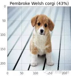
print("Predicted class is #{}.".format(out['prob'][0].argmax()))

That’s it! Just 3 lines of code. Similarly, I can classify an adorable puppy!

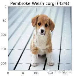
It turns out this dog is not a corgi, just very similar in color. This network indeed knows more about dogs than I do.

What a Mistake Looks Like (Using the Queen as an Example)

The most interesting thing while doing this work is that I discovered what the neural network thinks the British Queen is wearing on her head.

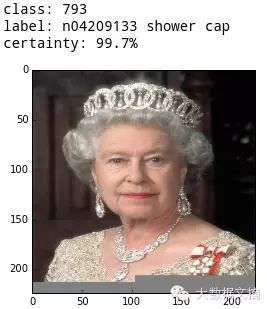
So now we see the network doing something right, while we also see it inadvertently making a cute mistake (the Queen is wearing a shower cap). Now… we let it intentionally make mistakes and dive into its core.

Intentionally Making Mistakes

Before truly understanding how it works, we need to perform some mathematical transformations. First, let’s look at its descriptions of a black screen.

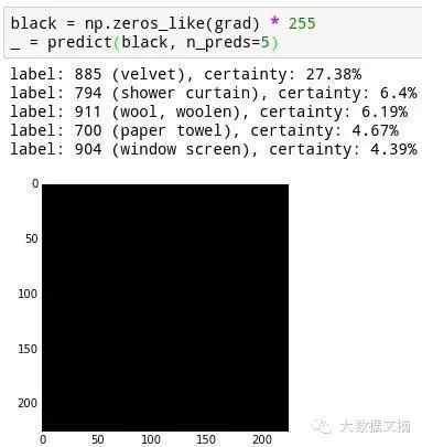
This pure black image is considered to have a 27% probability of being velvet and a 4% probability of being a paper towel. There are other category probabilities not listed, totaling 100%.

I want to figure out how to make the neural network more confident that this is a paper towel.

To do this, we need to calculate the gradient of the neural network, which is the derivative of the neural network. You can think of this as a direction that makes the image look more like a paper towel in that direction.

To calculate the gradient, we first need to choose an intended outcome to move towards and set the output probability list, where 0 indicates any direction and 1 indicates the direction of a paper towel. The backpropagation algorithm is a method for calculating gradients. I thought it was mysterious, but in fact, it’s just an algorithm that implements the chain rule.

Below is the code I wrote, which is actually very simple! Backpropagation is one of the most basic neural network operations, so it is readily available in libraries.

def compute_gradient(image, intended_outcome):
    # Put the image into the network and make the prediction
    predict(image)
    # Get an empty set of probabilities
    probs = np.zeros_like(net.blobs['prob'].data)
    # Set the probability for our intended outcome to 1
    probs[0][intended_outcome] = 1
    # Do backpropagation to calculate the gradient for that outcome
    # and the image we put in
    gradient = net.backward(prob=probs)
    return gradient['data'].copy()

This basically tells us what kind of neural network will be looking for at this point. Since everything we deal with can be represented as an image, below is the output of compute_gradient(black, paper_towel_label), scaled to a visible proportion.

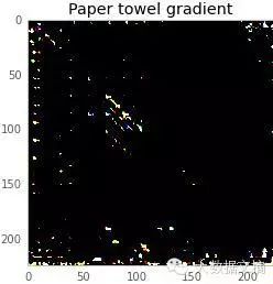
Now, we can add or subtract a very bright portion from our black screen to make the neural network think our image looks more or less like a paper towel. Since the image we added is too bright (pixel values less than 1 / 256), the difference is not visible at all. Below is this result:

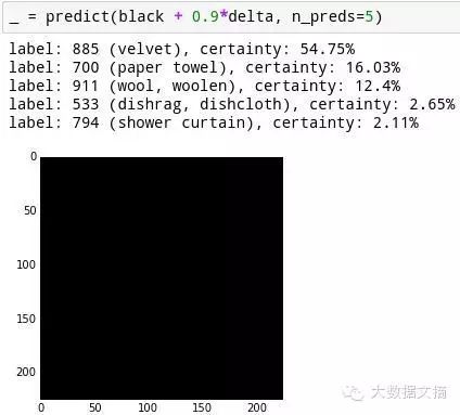
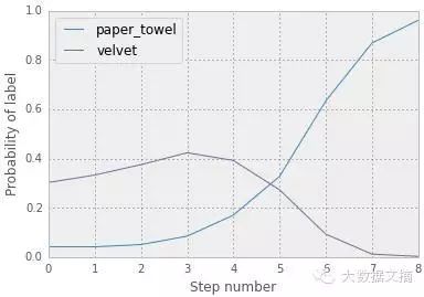
Now, the neural network is 16% sure that our black screen is a paper towel, instead of 4%! Very clever. But we can do better. We can take ten small steps to construct an image that looks somewhat like a paper towel at each step, rather than taking a direct step in the direction of a paper towel. You can see the probability changing over time below. You will notice that the probability values differ from before because our step size is different (0.1 instead of 0.9).

Final Result:

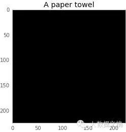
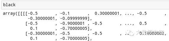
Below are the pixel values that make up this image! They all start from 0, and you can see that we have transformed them to make the neural network believe that this image is a paper towel.

We can also multiply this image by 50 to achieve a better image perception.

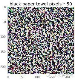
To me, this doesn’t look like a paper towel, but it might to you. I suspect all the swirls in the image tricked the neural network into thinking this is a paper towel. This involves basic proof of concept and some mathematical principles. Soon, we will delve into more mathematical knowledge, but first, let’s have some fun.

Playing with Neural Networks

Once I understood this, it became very interesting. We can transform a cat into a bath towel:

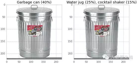
A trash can can become a kettle/cocktail shaker:

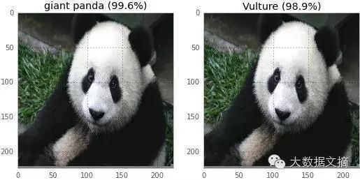
A panda can become a vulture.

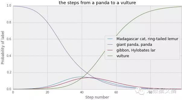
This chart shows that within 100 steps of making the panda think it is a vulture, the probability curve changes rapidly.

You can check the code to run these in the IPython notebook. It’s really fun.

Now, it’s time for a bit more mathematical principles.

How It Works: Logistic Regression

First, let’s discuss the simplest method of image classification – logistic regression. What is logistic regression? Let me try to explain.

Suppose you have a linear function to classify whether an image is a raccoon. So how do we use a linear function? Now suppose your image has only 5 pixels (x1, x2, x3, x4, x5), with values between 0 and 255. Our linear function has weights, say (23, -3, 9, 2, 5), then we classify the image, and we will get the inner product of the pixels and weights:

result=23×1−3×2+9×3+2×4−5×5

Suppose the result is 794. So what does 794 mean? Is it a raccoon or not? 794 is not a probability, of course. Probability is a number between 0 and 1. Our result is between −∞ and ∞. A common method to convert a number from −∞ to ∞ into a probability value is to use a function called logistic: S(t)=1/(1+e^(-t))

The graph of this function is as follows:

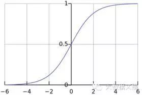
The result of S(794) is basically 1, so if we get 794 from the raccoon weights, then we can be 100% sure it is a raccoon. In this model – we first use a linear function to transform the data, and then apply the logistic function to get a probability value. This is logistic regression, and it is a very simple and popular machine learning technique.

The “learning” in machine learning mainly refers to how to determine the correct weights (such as (23, -3, 9, 2, 5)) under a given training set, so that the probability values we obtain can be as good as possible. Usually, the larger the training set, the better.

Now that we understand what logistic regression is, let’s discuss how to break it!

Breaking Logistic Regression

There is a splendid blog post by Andrej Karpathy titled “Breaking Linear Classifiers on ImageNet,” which explains how to perfectly break a simple linear model (not logistic regression, but a linear model). Later, we will use the same principle to break neural networks.

Here is an example (from Karpathy’s article), visualizing some linear classifiers that distinguish different foods, flowers, and animals as shown in the figure (click to enlarge).

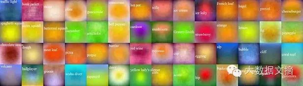
You can see that the “Granny Smith” classifier basically asks, “Is it green?” (not in the worst way to find out!), while the “menu” classifier finds that menus are usually white. Karpathy explains this very clearly:

For example, apples are green, so the linear classifier presents positive weights on the green channel and negative weights on the blue and red channels across all spatial locations. Therefore, it effectively calculates the amount of green components in the middle.

So if I want the Granny Smith classifier to think I am an apple, what I need to do is:

• Find out which pixel in the image cares most about green

• Color the pixel that cares about green

• Done!

So now we know how to deceive a linear classifier. But neural networks are not linear; they are highly nonlinear! Why is this relevant?

How It Works: Neural Networks

I have to be honest here: I am not a neural network expert, and my explanation of neural networks won’t be outstanding. Michael Nielsen has written a great book called “Neural Networks and Deep Learning.” Additionally, Christopher Olah’s blog is also good.

What I know about neural networks is that they are functions. You input an image, and you get a list of probabilities, one for each class. These are the numbers you see for the images in this article. (Is it a dog? No. A shower cap? No. A solar panel? YES!!)

Therefore, a neural network is like 1000 functions (each probability corresponds to one). But 1000 functions are very complex for reasoning. Thus, people who create neural networks combine these 1000 probabilities into a single “score,” which is called a “loss function.”

The loss function for each image depends on the actual correct output of the image. Suppose I have a picture of an ostrich, and the neural network has an output probability Pj, where j=1…1000, but for each ostrich, I want the probability to be yj. Then the loss function is:

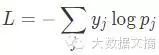
Assuming the label value corresponding to “ostrich” is 700, then y700=1, and the others yj will be 0, L=-logp700.

The key point here is to understand that the neural network gives you a function, and when you input an image (panda), you get the final value of the loss function (a number, like 2). Since it is a single-valued function, we assign the derivative (or gradient) of that function to another image. Then you can use this image to deceive the neural network, using the method we discussed earlier in this article!

Breaking Neural Networks

Below is about how to relate breaking a linear function/logistic regression to breaking neural networks! This is the mathematical principle you’ve been waiting for! Think about our image (the cute panda), the loss function looks like:

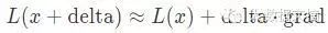
Where the gradient grad equals ∇L(x). Because this is calculus. To make the loss function change more, we want to maximize the dot product of the delta we move and the gradient grad. Let’s calculate the gradient using the compute_gradient() function and draw it as an image:

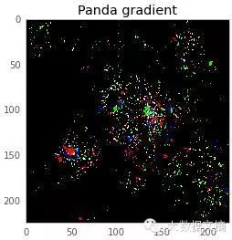
Intuitively, we need to create a delta that emphasizes the pixels in the image that the neural network thinks are important. Now, suppose grad is (−0.01, −0.01, 0.01, 0.02, 0.03).

We can take delta=(−1, −1, 1, 1, 1), then grad⋅delta equals 0.08. Let’s try it! In code, it’s delta = np.sign(grad). When we move by this amount, sure enough – now the panda turns into a ferret.

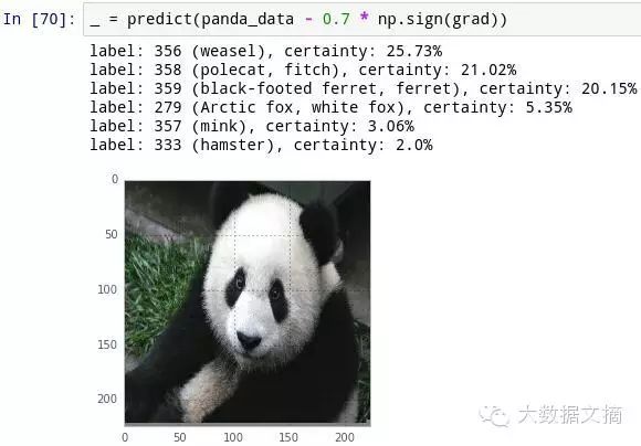
But why? Let’s think about the loss function we started seeing. It shows that the probability of it being a panda is 99.57%. −log(0.9957)=0.0018. Very small! Therefore, adding a delta will increase our loss function (making it less like a panda), while subtracting a delta will decrease our loss function (making it more like a panda). But the fact is exactly the opposite! I’m still confused about this.

You Can’t Deceive a Dog

Now that we understand the mathematical principles, a brief description. I also tried to deceive the network into recognizing that previously cute puppy:

But for the dog, the network strongly resisted classifying it as anything other than a dog! I spent some time trying to make it believe that the dog was a tennis ball, but it remained a dog. A different kind of dog! But still a dog.

I met Jeff Dean (who works on neural networks at Google) at a conference and asked him about this. He told me that this network has a bunch of dogs in the training set, more than pandas. So he assumes that it’s about training a better network to recognize dogs. That seems reasonable!

I find this very cool, and it makes me feel like training more precise networks is more promising.

There’s another interesting thing about this topic – when I tried to make the network think that the panda was a vulture, it took a little time deciding whether it was an ostrich. When I asked Jeff Dean about the panda and dog question, he casually mentioned the “panda-ostrich space,” and I hadn’t mentioned that the network had considered whether the panda was an ostrich when thinking it was a vulture. This is really cool; he clearly knows that pandas and ostriches are closely related in some way by using data and these networks.

Less Mystery

When I started doing this, I hardly knew what a neural network was. Now I can make it think a panda is a vulture and see how cleverly it classifies dogs, and I understand them a little bit. I no longer think what Google is doing is magical, but I am still puzzled by neural networks. There is so much to learn! Using this method to deceive them removes some of the mystery, and now I have more understanding of them.

I believe you can too! All the code for this program is in the neural-networks-are-weird repository. It uses Docker, so you can easily install it, and you don’t need a GPU or a new computer. This code runs on my old GPU laptop that I’ve been using for 3 years.

To learn more, read the original paper: “Explaining and Harnessing Adversarial Examples.” The paper is short, well-written, and will tell you more that this article did not cover, including how to use this technique to build better neural networks!

Finally, thanks to Mathieu Guay-Paquet, Kamal Marhubi, and others who helped me in writing this article!

[Limited-Time Resource Download]

Click the image below to read “7 Major Trends in Big Data Development in 2016”

Before January 31, 2016

For the December 2015 resource package download, please click the bottom menu of Big Data Digest: Download etc. — December Download

Wonderful articles from Big Data Digest:

Reply with 【Finance】 to see historical journal articles from the Finance and Business column

Reply with 【Visualization】 to experience the perfect combination of technology and art

Reply with 【Security】 for fresh cases about leaks, hacking, and offense and defense

Reply with 【Algorithm】 for interesting people and events that expand knowledge

Reply with 【Google】 to see its initiatives in the field of big data

Reply with 【Academician】 to see how many academicians talk about big data

Reply with 【Privacy】 to see how much privacy remains in the era of big data

Reply with 【Medical】 to check out 6 articles in the medical field

Reply with 【Credit】 for four articles on big data credit

Reply with 【Great Power】 “Big Data National Archives” of the United States and 12 other countries

Reply with 【Sports】 to see application cases of big data in tennis, NBA, etc.

Reply with 【Volunteer】 to learn how to join Big Data Digest

Long press the fingerprint to follow “Big Data Digest”

Focusing on big data, sharing daily