

1 Compiled by New Intelligence Source
Author: Alberto Quesada
Source: neuraldesigner.com
Translated by: Liu Xiaoqin
[New Intelligence Source Guide] There are thousands of algorithms for training neural networks. Which ones are the most commonly used, and which is the best? The author introduces five common algorithms in this article and compares them in terms of memory and speed. Finally, he recommends the Levenberg-Marquardt algorithm.
The programs used to execute the learning process in neural networks are called training algorithms. There are many training algorithms, each with different characteristics and performance.
The learning problem in neural networks is defined by the minimization of the loss function f. This function generally consists of an error term and a regularization term. The error term evaluates how well the neural network fits the dataset, while the regularization term is used to prevent overfitting by controlling the effective complexity of the neural network.
The loss function depends on the adaptive parameters in the neural network (biases and synaptic weights). We can conveniently combine them into a single n-dimensional weight vector w. The following diagram represents the loss function f(w)

As shown in the figure above, the point w* is the minimum of the loss function. At any point A, we can calculate the first and second derivatives of the loss function. The first derivative consists of the gradient vector and can be written as:
ᐁif(w) = df/dwi (i = 1,…,n)
Similarly, the second derivative of the loss function can be expressed using the Hessian matrix as:
Hi,jf(w) = d2f/dwi·dwj (i,j = 1,…,n)
Many minimization problems for continuous and differentiable functions have been extensively studied. The conventional methods for these problems can be directly applied to training neural networks.
Although the loss function depends on many parameters, one-dimensional optimization methods are very important here. In fact, one-dimensional optimization methods are often used in the training process of neural networks.
Many training algorithms first compute the training direction d, then calculate the training rate η that minimizes the loss along that direction, written as f(n). The following diagram describes the one-dimensional loss function:
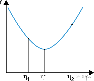
The points η1 and η2 define the interval containing the minimum η* of f(n). Here, the one-dimensional optimization method searches for the minimum of a given one-dimensional function. Commonly used algorithms include the golden section method and Brent’s method.
The learning problem in neural networks is defined as the search for the parameter vector w* that minimizes the loss function f. If the loss function of the neural network has already reached a minimum, then the gradient is a zero vector.
In general, the loss function is a nonlinear function of the parameters. Therefore, it is impossible to find a closed training algorithm for the minimum. Instead, we consider searching for the minimum in a parameter space composed of a series of steps. At each step, the loss decreases as the parameters of the neural network are adjusted.
Thus, we start training the neural network from some parameter vector (usually chosen randomly). We then generate a series of parameters such that the loss function decreases in each iteration of the algorithm. The change in loss between two iterations is called the loss reduction. The training algorithm stops when specific conditions are met or a stopping criterion is reached.
The next section will introduce the five most important algorithms for training neural networks.

Gradient descent, also known as the steepest descent method, is the simplest training algorithm. It requires information from the gradient vector, thus it is a first-order method.
Let f(wi) = fi,ᐁf(wi) = gi. The method starts from point w0 and moves from wi to wi+1 in the training direction di = -gi until the stopping criteria are met. Thus, the gradient descent method iterates according to the following formula:
wi+1 = wi – di·ηi, i=0,1,…
Here, the parameter η is the training rate. This value can be set as a fixed value or found through one-dimensional optimization at each step along the training direction. The optimal value for the training rate is usually obtained through linear minimization at each successive step. However, many software tools still use a fixed training rate.
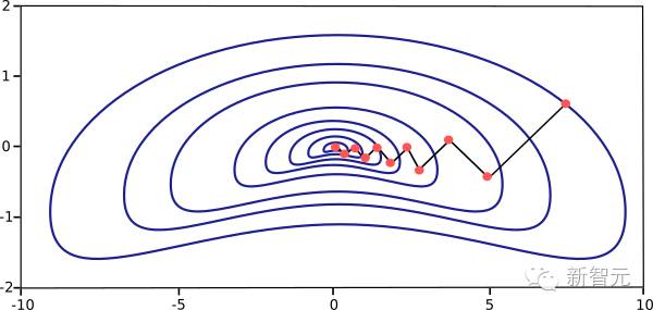
The following diagram illustrates the training process of gradient descent. It can be seen that the parameter vector is enhanced in two steps: first, calculating the gradient descent training direction; then, finding the appropriate training rate.

The major drawback of the gradient descent training algorithm is that it requires many iterations for functions with long and narrow valley structures. In practice, the down-slope gradient is the direction of fastest descent of the loss function, but it does not necessarily produce the fastest convergence. The following diagram illustrates this problem.
When the neural network is very large and has many parameters, gradient descent is the recommended algorithm. This is because this method only stores the gradient vector (size n) and does not store the Hessian matrix (size n2).
Newton’s method is a second-order algorithm because it uses the Hessian matrix. The goal of this method is to find a better training direction by using the second derivative of the loss function.
Let f(wi) = fi, ᐁf(wi) = gi, and Hf(wi)= Hi. Using Taylor series, we obtain a quadratic approximation of f at w0:
f = f0 + g0 · (w – w0) + 0.5 · (w – w0)2 · H0
H0 is the Hessian matrix of f estimated at point w0. By setting g=0 for the minimum of f(w), we obtain the following equation:
g = g0 + H0 · (w – w0) = 0
Thus, starting from the parameter vector w0, Newton’s method iterates according to the following formula:
wi+1 = wi – Hi-1·gi, i=0,1,…
The vector Hi-1·gi is called the Newton step. It is important to note that these parameter changes may move towards a maximum rather than a minimum. This occurs if the Hessian matrix is not positive definite. Therefore, it cannot be guaranteed that the function value decreases with each iteration. To avoid this issue, the equation of Newton’s method is usually modified to:
wi+1 = wi – (Hi-1·gi)·ηi, i=0,1,…
The training rate η can be set as a fixed value or found through linear minimization. The vector d = Hi-1·gi is now referred to as the Newton training direction.
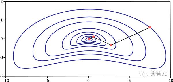
The training process of Newton’s method is illustrated in the following diagram, where the Newton training direction is first obtained, followed by finding an appropriate training rate to perform parameter improvements.

The following diagram describes the performance of this method. It can be seen that Newton’s method requires fewer gradient descent steps than those required to find the minimum of the loss function.
However, the drawback of Newton’s method is that it is computationally expensive to accurately estimate the Hessian matrix and its inverse matrix.
The conjugate gradient method can be considered as a method that lies between gradient descent and Newton’s method. It can accelerate the typical slow convergence of gradient descent while avoiding the need for the evaluation, storage, and inversion of the Hessian matrix required by Newton’s method.
In the conjugate gradient training algorithm, the search is performed along conjugate directions, which typically lead to faster convergence than the gradient descent direction. These training directions are related to the Hessian matrix.
Let d represent the training direction vector. Then, starting from the initial parameter vector w0 and the initial training direction vector d0 = -g0, the conjugate gradient method constructs a sequence of training directions represented as:
di+1 = gi+1 + di·γi, i=0,1,…
Here, γ is called the conjugate parameter and has different calculation methods. Two of the most commonly used methods are Fletcher-Reeves and Polak-Ribière. For all conjugate gradient algorithms, the training direction is periodically reset to the negative value of the gradient.
Then, the parameters are improved according to the following equation, where the training rate η is usually obtained through linear minimization:
wi+1 = wi + di·ηi, i=0,1,…
The following diagram describes the training process using the conjugate gradient method. As shown, the steps for parameter improvement first calculate the conjugate gradient training direction and then calculate the appropriate training rate along that direction.

This method has proven to be more effective than gradient descent for training neural networks. Since it does not require the Hessian matrix, it is also recommended when the neural network is very large.
Newton’s method is computationally quite expensive because it requires many operations to evaluate the Hessian matrix and compute its inverse. To address this drawback, an alternative method known as the quasi-Newton method or variable matrix method has emerged. This method builds and approximates the inverse Hessian matrix at each iteration of the algorithm, rather than calculating the Hessian matrix directly and then evaluating its inverse. This approximation uses only first-order derivative information from the loss function.
The Hessian matrix consists of the second-order partial derivatives of the loss function. The main idea behind the quasi-Newton method is to approximate the inverse Hessian matrix using only the first-order partial derivatives of the loss function through another matrix G. The formula for the quasi-Newton method can be expressed as:
wi+1 = wi – (Gi·gi)·ηi, i=0,1,…
The training rate η can be set as a fixed value or found through linear minimization. The two most commonly used formulas are the Davidon-Fletcher-Powell (DFP) formula and the Broyden-Fletcher-Goldfarb-Shanno (BFGS) formula.
The training process of the quasi-Newton method is illustrated in the following diagram. First, the quasi-Newton training direction is obtained, and then a satisfactory training rate is found to perform parameter improvements.

This is the default method used in most cases: it is faster than both gradient descent and conjugate gradient methods and does not require precise calculation and inversion of the Hessian matrix.
5. Levenberg-Marquardt Algorithm
The Levenberg-Marquardt algorithm, also known as the damped least squares method, is designed to use a specific algorithm for loss functions in the form of the sum of squared errors. It does not require precise calculation of the Hessian matrix and is suitable for gradient vectors and Jacobian matrices.
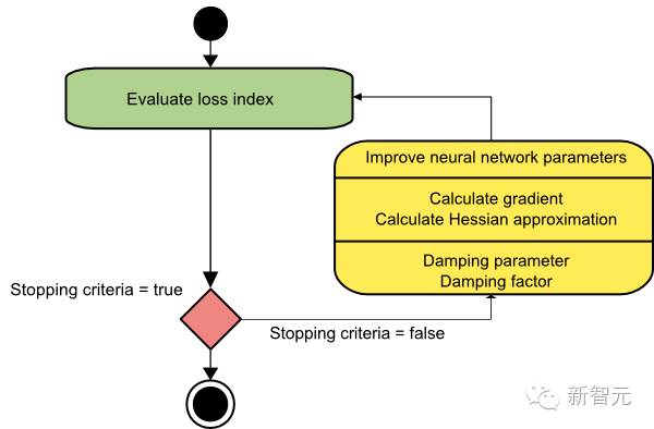
The following diagram illustrates the neural network training process using the Levenberg-Marquardt algorithm. The first step is to calculate the loss value, gradient, and Hessian approximation, and then adjust the damping parameter to reduce the loss in each iteration.
The Levenberg-Marquardt algorithm is a specific method for functions of the sum of squared errors. This makes it very fast when measuring such errors in training neural networks. However, the algorithm also has some drawbacks. One of the drawbacks is that it cannot be applied to functions such as root mean square error or cross-entropy loss functions. Additionally, it is incompatible with regularization terms. Finally, for very large datasets and neural networks, the Jacobian matrix becomes very large, thus requiring a lot of memory. Therefore, when the dataset and/or neural network is very large, the Levenberg-Marquardt algorithm is not recommended.
The following diagram compares the computational speed and storage requirements of the training algorithms discussed in this article. It can be seen that the slowest training algorithm is gradient descent, but it requires the least memory. In contrast, the fastest is the Levenberg-Marquardt algorithm, but it also requires the most memory. A good compromise may be the quasi-Newton method.
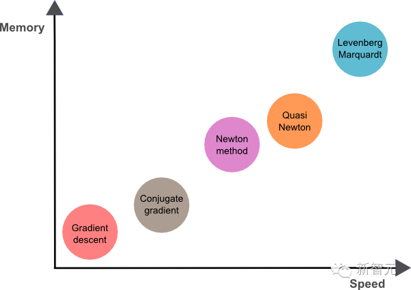
In summary, if our neural network has thousands of parameters, we can use gradient descent or conjugate gradient methods to save memory. If the neural network we want to train has only a few thousand samples and hundreds of parameters, the best choice may be the Levenberg-Marquardt algorithm. In other cases, the quasi-Newton method can be chosen.


Click to read the original text and watch the full video recap of the 2016 World Artificial Intelligence Conference main forum.