Click the above“Beginner Learning Vision” and choose to add “Star” or “Top“
Important content delivered promptly
Important content delivered promptlyAuthor丨Linglong@Zhihu (Authorized)Source丨https://zhuanlan.zhihu.com/p/577295030Editor丨Jishi Platform
Jishi Guide
This article first introduces the automatic differentiation method of computational graphs, then derives the gradients of Kernel and Input in convolution operations, and subsequently implements the convolution operator based on Pytorch and performs correctness verification.
Introduction
This article has two main purposes:
- Derive the gradient formulas for various variables involved in convolution operations;
- Learn how to extend Pytorch operators, implementing a convolution operator that can perform forward and backward passes;
First, the automatic differentiation method of computational graphs is introduced, followed by the derivation of gradients for Kernel and Input in convolution operations, and finally, the implementation of the convolution operator based on Pytorch and correctness verification.
The code for this article can be found in this GitHub repository: https://github.com/dragonylee/myDL/blob/master/%E6%89%A9%E5%B1%95%E6%B5%8B%E8%AF%95.ipynb.
Computational Graph
A computational graph (Computational Graph) is the theoretical basis for torch.autograd automatic differentiation, described as a directed acyclic graph (DAG), where the direction of the arrows represents the forward propagation direction, while the reverse direction represents the backward propagation process, allowing for easy calculation of partial derivatives for any variable. To illustrate, here is a simple example:
Where is the input, and is the output.
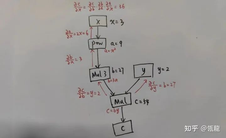
According to the chain rule, we can obtain:
Define the above three functions in Pytorch (Python):
def square(x):
    return x ** 2

def mul3(x):
    return x * 3

def mul_(x, y):
    return x * y
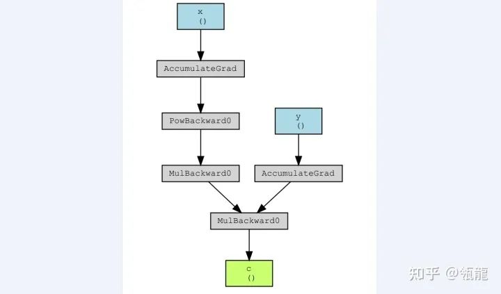
Then use torchviz to visualize the computational graph of the composite function:
x = torch.tensor(3., requires_grad=True, dtype=torch.float)
y = torch.tensor(2., requires_grad=True, dtype=torch.float)
a = square(x)   # a=x^2
b = mul3(a)     # b=3a
c = mul_(b, y)  # c=by

torchviz.make_dot(c, {"x": x, "y": y, "c": c}).view()
The following result is obtained:
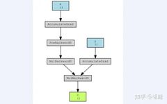
Ignoring the operation “Accumulate”, the backward differentiation process on this computational graph is represented as follows:
This clearly demonstrates the function of the computational graph, which records the computation functions of each variable (including outputs and intermediate variables) (which can be referred to as an operator, represented by the boxes in the graph, where incoming edges are inputs and outgoing edges are outputs), allowing for numerical computation of the corresponding derivatives. In fact, the derivative of any variable qqq with respect to ppp can be obtained by multiplying the backward links between the two.
After calling .backward() on the output, the derivative values can be viewed:
c.backward()
print(y.grad)
print(x.grad)
The output results are consistent with the computational results shown above. Note that during the backward process, non-leaf nodes can call .retain_grad() to record grad.
I used to think that automatic differentiation was a very complex operation, but I didn’t expect a computational graph to implement it so simply. I realized that what I thought was a complex operation was actually a formalized differentiation…
Convolution Operations and Gradient Derivation
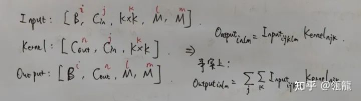
The convolution operation discussed in this article is the most basic convolution operation, without stride, padding, dilation, bias, etc. The convolution operation is defined as
Output Input Kernel,
where is the input, Kernel is the convolution kernel, Output Tensor is the output, and has .
How to Implement Convolution?
You can first use nn.Unfold to unfold the input tensor. Note that Unfold() can also specify stride, dilation, etc., but we will not consider these here, so we can just pass in kernel_size to unfold the Input into Tensor form.
input_unf = nn.Unfold(kernel_size=K)(input)
Then use view to convert the Input into Tensor form.
input_unf = input_unf.view((B, Cin, -1, M, M))
Similarly, convert the Kernel into Tensor form using view.
kernel_view = kernel.view((Cout, Cin, K * K))
And the output Output is in Tensor form.
At this point, the convolution operation can be directly written using Einstein summation notation:
The code is
output = torch.einsum("ijklm,njk->inlm", input_unf, kernel_view)
How to Calculate Gradients?
The derivation of this part was completed by me on draft paper, and after some verification, it should be guaranteed to be correct.
To use Pytorch’s built-in gradcheck to verify the correctness of backward gradient calculations, we need to differentiate each input parameter. Assuming the final Loss function result is (a scalar), we need to calculate the derivative of Input and the derivative of the convolution kernel Kernel .
For convenience in derivation, we will not consider batch and channel, meaning Input, Kernel, and Output are all two-dimensional.
Gradient of Kernel
According to the chain rule, we can express this derivative (partial derivative) as
In which is known (it will be passed along as a parameter during the backward process), which is the product of all gradients along the chain link behind the current convolution operator in the computational graph, and its size is consistent with Output.
The question then is to find the partial derivative of Output with respect to Kernel, we can derive it using a simple example:
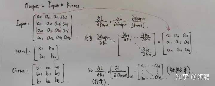
It can be found that is actually the dot product of and the top-left submatrix of the Input matrix. The same applies to other , thus we can conclude:
In other words, the gradient of Kernel is the result of convolving the gradient of Output with the Input as the kernel.
Gradient of Input
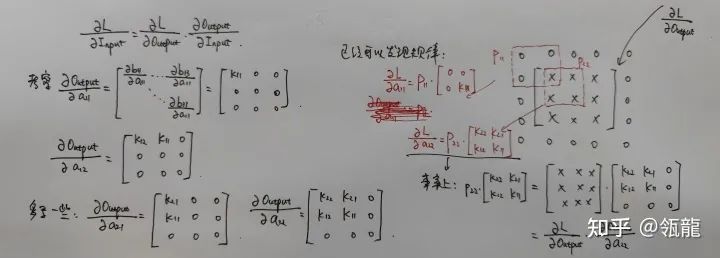
We can find that by appropriately padding with 0, convolving with the rotated Kernel gives us . The formula can be expressed as (may not be very standard):

Thus, the calculation method for the gradient of Input can be expressed as: the gradient of Input is the result of convolving with the rotated 180° Kernel as the kernel for the deconvolution of .
Custom Convolution Operator
A major purpose of this article is to learn how to extend Pytorch operators. According to the official documentation, it is necessary to implement a function that inherits torch.autograd.Function and implement the static functions forward and backward to adapt to Pytorch’s automatic differentiation framework. There are some details to note:
forwardandbackwardfunctions both have the first parameter asctx, which means context, similar toself. If parameters from forward are needed in backward,ctx.save_for_backward()should be called during forward to save them;forwardhas as many inputs asbackwardhas outputs, which can be understood from the computational graph. If an input edge does not require gradient,Nonecan be returned;
Gradient Calculation
Previously, when defining the convolution operation, we considered Batch and Channel, while in deriving the gradients for Input and Kernel, we did not consider these two parameters for convenience. In practice, it is crucial to pay special attention to the relationship between each dimension in the view of each data.
For example, I define:
Input : Tensor Kernel: Tensor Output: Tensor
When calculating the gradient of Kernel, according to the formula Input , the dimensions here are
Input: Tensor Tensor Tensor
Therefore, we need to first swap the 01 dimensions of Input (transpose), then swap the 01 dimensions of , and then perform convolution, and the result needs to swap the 01 dimensions again to obtain . The code is written as:
input_ = torch.transpose(input, 0, 1)
grad_output_ = torch.transpose(grad_output, 0, 1)
grad_weight = MyConv2dFunc.conv2d(input_, grad_output_).transpose(0, 1)
The calculation of the gradient for Input is similar.
Code
class MyConv2dFunc(torch.autograd.Function):
    @staticmethod
    def conv2d(input: Tensor, kernel: Tensor) -> Tensor:
        """
            Convolution operation
            Output = Input * Kernel
        :param input: Tensor[B, Cin, N, N]
        :param kernel: Tensor[Cout, Cin, K, K]
        :return: Tensor[B, Cout, M, M], M=N-K+1
        """
        B = input.shape[0]
        Cin = input.shape[1]
        N = input.shape[2]
        Cout = kernel.shape[0]
        K = kernel.shape[2]
        M = N - K + 1

        input_unf = nn.Unfold(kernel_size=K)(input)
        input_unf = input_unf.view((B, Cin, -1, M, M))
        kernel_view = kernel.view((Cout, Cin, K * K))

        output = torch.einsum("ijklm,njk->inlm", input_unf, kernel_view)
        return output

    @staticmethod
    def forward(ctx, input, weight):
        ctx.save_for_backward(input, weight)
        output = MyConv2dFunc.conv2d(input, weight)
        return output

    @staticmethod
    def backward(ctx, grad_output):
        input, weight = ctx.saved_tensors
        grad_input = grad_weight = None
        if grad_output is None:
            return None, None
        if ctx.needs_input_grad[0]:
            # Deconvolution
            gop = nn.ZeroPad2d(weight.shape[2] - 1)(grad_output)
            kk = torch.rot90(weight, 2, (2, 3))  # Rotate 180 degrees
            kk = torch.transpose(kk, 0, 1)
            grad_input = MyConv2dFunc.conv2d(gop, kk)
        if ctx.needs_input_grad[1]:
            input_ = torch.transpose(input, 0, 1)
            grad_output_ = torch.transpose(grad_output, 0, 1)
            grad_weight = MyConv2dFunc.conv2d(input_, grad_output_).transpose(0, 1)
        return grad_input, grad_weight
Correctness Verification
torch.autograd.gradcheck provides a tool for verifying the correctness of gradient operations. Its principle is to compute a Jacobian matrix of output and input using the backward calculation of your operator with given inputs, and then calculate a numerical solution using the finite difference method, and compare whether these two results are consistent.
Verify the correctness of the MyConv2dFunc operator:
input = (torch.rand((2, 4, 10, 10), requires_grad=True, dtype=torch.double),
             torch.rand((6, 4, 5, 5), requires_grad=True, dtype=torch.double))
test = torch.autograd.gradcheck(MyConv2dFunc.apply, input)
print(test)
The output is True.
Custom Convolution Layer Model
It needs to inherit nn.Module and use nn.Parameter to store weights, which are the convolution kernels. The forward method must also be implemented.
class MyConv2d(nn.Module):
    def __init__(self, in_channels, out_channels, kernel_size: tuple):
        super(MyConv2d, self).__init__()
        self.in_channels = in_channels
        self.out_channels = out_channels
        self.kernel_size = kernel_size
        # Parameters
        self.weight = nn.Parameter(torch.empty(out_channels, in_channels, kernel_size[0], kernel_size[1]))

        nn.init.uniform_(self.weight, -0.1, 0.1)

    def forward(self, x):
        return MyConv2dFunc.apply(x, self.weight)

    def extra_repr(self):
        return 'MyConv2d: in_channels={}, out_channels={}, kernel_size={}'.format(
            self.in_channels, self.out_channels, self.kernel_size
        )
Testing Based on MNIST
The convolutional neural network model used is LeNet:
CNN(
  (layer1): Sequential(
    (0): Conv2d(1, 32, kernel_size=(3, 3), stride=(1, 1))
    (1): ReLU()
    (2): Conv2d(32, 64, kernel_size=(3, 3), stride=(1, 1))
    (3): BatchNorm2d(64, eps=1e-05, momentum=0.1, affine=True, track_running_stats=True)
    (4): ReLU()
    (5): MaxPool2d(kernel_size=2, stride=2, padding=0, dilation=1, ceil_mode=False)
  )
  (flatten): Flatten(start_dim=1, end_dim=-1)
  (fc): Sequential(
    (0): Linear(in_features=9216, out_features=256, bias=True)
    (1): ReLU()
    (2): Linear(in_features=256, out_features=10, bias=True)
  )
)
The task is to classify MNIST handwritten digits.
First, use Pytorch’s built-in Conv, Linear, and other network layers to build and train, then replace the Conv2d in the network with my MyConv2d and perform the same training, obtaining the following results (5 epochs, CUDA):
| Accuracy | Time Cost(s) | |
|---|---|---|
| nn.Conv2d | 99.2% | 33.72 |
| MyConv2d | 99.1% | 76.49 |
Download 1: OpenCV-Contrib Extension Module Chinese Tutorial

Reply "Extension Module Chinese Tutorial" in the backend of the "Beginner Learning Vision" public account to download the first Chinese OpenCV extension module tutorial on the internet, covering installation of extension modules, SFM algorithms, stereo vision, object tracking, biological vision, super-resolution processing, etc. over twenty chapters of content.

Download 2: Python Vision Practical Project 52 Lectures

Reply "Python Vision Practical Project" in the backend of the "Beginner Learning Vision" public account to download 31 practical vision projects including image segmentation, mask detection, lane line detection, vehicle counting, adding eyeliner, license plate recognition, character recognition, emotion detection, text content extraction, face recognition, etc., to assist in quickly learning computer vision.

Download 3: OpenCV Practical Project 20 Lectures

Reply "OpenCV Practical Project 20 Lectures" in the backend of the "Beginner Learning Vision" public account to download 20 practical projects based on OpenCV, achieving advanced learning of OpenCV.

Discussion Group

Welcome to join the reader group of the public account to communicate with peers. Currently, there are WeChat groups for SLAM, 3D vision, sensors, autonomous driving, computational photography, detection, segmentation, recognition, medical imaging, GAN, algorithm competitions, etc. (these will gradually be subdivided). Please scan the WeChat ID below to join the group, and note: "Nickname + School/Company + Research Direction", for example: "Zhang San + Shanghai Jiaotong University + Vision SLAM". Please follow the format when noting; otherwise, you will not be approved. After successfully adding, you will be invited into relevant WeChat groups based on your research direction. Please do not send advertisements in the group; otherwise, you will be removed. Thank you for your understanding~