Selected from GitHub
Compiled by Machine Heart
Contributors: Geek.ai, Siyuan
PyTorch is one of the best deep learning frameworks, known for its simplicity and elegance, making it ideal for beginners. This article will introduce the best practices and coding styles for PyTorch.
Although this is an unofficial PyTorch guide, the article summarizes over a year of experience using the PyTorch framework, especially the optimal solutions developed for deep learning-related tasks. Please note that most of the shared experiences are derived from research and practical perspectives.
This is a developing project, and other readers are welcome to improve the document: https://github.com/IgorSusmelj/pytorch-styleguide.
The document mainly consists of three parts: first, we will briefly outline the best tools in Python. Next, we will introduce some tips and suggestions for using PyTorch. Finally, we will share insights and experiences from using other frameworks that typically help us improve our workflow.
Outlining Python Tools
It is recommended to use Python version 3.6 or higher
Based on our experience, we recommend using Python version 3.6 or higher because they have the following features, which make it easier to write concise code:
-
Support for the ‘typing’ module since Python 3.6
-
Support for formatted strings (f-strings) since Python 3.6
Python Style Guide
We try to follow Google’s Python programming style. Please refer to Google’s excellent Python coding style guide:
Address: https://github.com/google/styleguide/blob/gh-pages/pyguide.md.
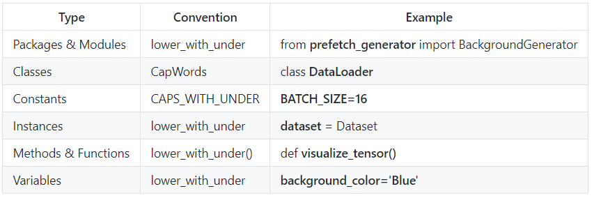
Here, we will provide a summary of the most commonly used naming conventions:
Integrated Development Environment
Generally, we recommend using integrated development environments like Visual Studio or PyCharm. VS Code provides syntax highlighting and auto-completion features among lightweight editors, while PyCharm has many advanced features for handling remote cluster tasks.
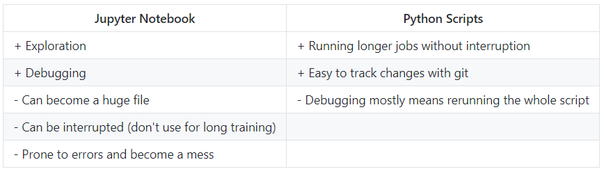
Jupyter Notebooks vs Python Scripts
Generally, we recommend using Jupyter Notebook for initial exploration or trying new models and code. If you want to train the model on larger datasets, you should use Python scripts, as reproducibility is more critical with larger datasets.
We recommend the following workflow:
-
In the initial stages, use Jupyter Notebook
-
Explore data and models
-
Build your classes/methods in notebook cells
-
Migrate the code to Python scripts
-
Train/deploy on the server
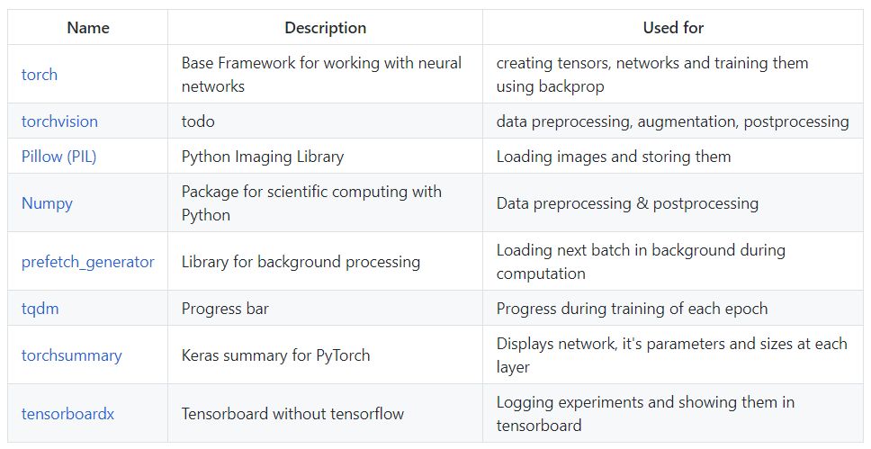
Common Libraries
Common libraries include:
File Organization
Do not put all layers and models in the same file. The best practice is to separate the final network into independent files (networks.py) and keep layers, loss functions, and various operations in their respective files (layers.py, losses.py, ops.py). The final model (composed of one or more networks) should be named after the model (for example, yolov3.py, DCGAN.py) and reference each module.
The main program, separate training, and testing scripts should only need to import the Python files with the model names.
PyTorch Development Style and Techniques
We recommend breaking down the network into smaller reusable segments. A nn.Module network contains various operations or other building modules. Loss functions are also included in nn.Module, allowing them to be directly integrated into the network.
Classes inheriting from nn.Module must have a ‘forward’ method that implements the forward propagation of various layers or operations.
A nn.Module can process input data through ‘self.net(input)’. Here, the object’s ‘call()’ method is directly used to pass input data to the module.
output = self.net(input)A Simple Network in PyTorch Environment
The following pattern can be used to implement a simple network with a single input and output:
class ConvBlock(nn.Module):
    def __init__(self):
        super(ConvBlock, self).__init__()
        block = [nn.Conv2d(...)]
        block += [nn.ReLU()]
        block += [nn.BatchNorm2d(...)]
        self.block = nn.Sequential(*block)

    def forward(self, x):
        return self.block(x)

class SimpleNetwork(nn.Module):
    def __init__(self, num_resnet_blocks=6):
        super(SimpleNetwork, self).__init__()
        # here we add the individual layers
        layers = [ConvBlock(...)]
        for i in range(num_resnet_blocks):
            layers += [ResBlock(...)]
        self.net = nn.Sequential(*layers)

    def forward(self, x):
        return self.net(x)
Please note the following points:
-
We reused simple loop building modules (like ConvBlocks), which consist of the same loop pattern (convolution, activation function, normalization) and packed into independent nn.Module.
-
We constructed a list of required layers and ultimately combined all layers into a model using ‘nn.Sequential()’. We used the ‘*’ operator before the list object to unpack it.
-
During forward propagation, we directly run the model with input data.
A Simple Residual Network in PyTorch Environment
class ResnetBlock(nn.Module):
    def __init__(self, dim, padding_type, norm_layer, use_dropout, use_bias):
        super(ResnetBlock, self).__init__()
        self.conv_block = self.build_conv_block(...)

    def build_conv_block(self, ...):
        conv_block = []

        conv_block += [nn.Conv2d(...),
                       norm_layer(...),
                       nn.ReLU()]
        if use_dropout:
            conv_block += [nn.Dropout(...)]

        conv_block += [nn.Conv2d(...),
                       norm_layer(...)]

        return nn.Sequential(*conv_block)

    def forward(self, x):
        out = x + self.conv_block(x)
        return out
Here, the skip connections of the ResNet module are directly implemented during forward propagation, allowing dynamic operations in PyTorch.
A Network with Multiple Outputs in PyTorch Environment
For networks with multiple outputs (for example, using a pre-trained VGG network to build perceptual loss), we use the following pattern:
class Vgg19(torch.nn.Module):
  def __init__(self, requires_grad=False):
    super(Vgg19, self).__init__()
    vgg_pretrained_features = models.vgg19(pretrained=True).features
    self.slice1 = torch.nn.Sequential()
    self.slice2 = torch.nn.Sequential()
    self.slice3 = torch.nn.Sequential()

    for x in range(7):
        self.slice1.add_module(str(x), vgg_pretrained_features[x])
    for x in range(7, 21):
        self.slice2.add_module(str(x), vgg_pretrained_features[x])
    for x in range(21, 30):
        self.slice3.add_module(str(x), vgg_pretrained_features[x])
    if not requires_grad:
        for param in self.parameters():
            param.requires_grad = False

  def forward(self, x):
    h_relu1 = self.slice1(x)
    h_relu2 = self.slice2(h_relu1)
    h_relu3 = self.slice3(h_relu2)
    out = [h_relu1, h_relu2, h_relu3]
    return out
Please note the following points:
-
We used pre-trained models provided by the ‘torchvision’ package
-
We split a network into three modules, each consisting of layers from the pre-trained model
-
We fixed the network weights by setting ‘requires_grad = False’
-
We returned a list with outputs from three modules
Custom Loss Functions
Even though PyTorch has a large number of standard loss functions, you may sometimes need to create your own loss function. To do this, you need to create a separate ‘losses.py’ file and create your custom loss function by extending ‘nn.Module’:
class CustomLoss(torch.nn.Module):

    def __init__(self):
        super(CustomLoss,self).__init__()

    def forward(self,x,y):
        loss = torch.mean((x - y)**2)
        return loss
Best Code Structure for Training Models
For the best code structure for training, we need to use the following two patterns:
-
Use BackgroundGenerator from prefetch_generator to load the next batch of data
-
Use tqdm to monitor the training process and display computational efficiency, which helps us identify bottlenecks in the data loading process
# import statements
import torch
import torch.nn as nn
from torch.utils import data
...

# set flags / seeds
torch.backends.cudnn.benchmark = True
np.random.seed(1)
torch.manual_seed(1)
torch.cuda.manual_seed(1)
...

# Start with main code
if __name__ == '__main__':
    # argparse for additional flags for experiment
    parser = argparse.ArgumentParser(description="Train a network for ...")
    ...
    opt = parser.parse_args()

    # add code for datasets (we always use train and validation/ test set)
    data_transforms = transforms.Compose([
        transforms.Resize((opt.img_size, opt.img_size)),
        transforms.RandomHorizontalFlip(),
        transforms.ToTensor(),
        transforms.Normalize((0.5, 0.5, 0.5), (0.5, 0.5, 0.5))
    ])

    train_dataset = datasets.ImageFolder(
        root=os.path.join(opt.path_to_data, "train"),
        transform=data_transforms)
    train_data_loader = data.DataLoader(train_dataset, ...)

    test_dataset = datasets.ImageFolder(
        root=os.path.join(opt.path_to_data, "test"),
        transform=data_transforms)
    test_data_loader = data.DataLoader(test_dataset ...)
    ...

    # instantiate network (which has been imported from *networks.py*)
    net = MyNetwork(...)
    ...

    # create losses (criterion in pytorch)
    criterion_L1 = torch.nn.L1Loss()
    ...

    # if running on GPU and we want to use cuda move model there
    use_cuda = torch.cuda.is_available()
    if use_cuda:
        net = net.cuda()
        ...

    # create optimizers
    optim = torch.optim.Adam(net.parameters(), lr=opt.lr)
    ...

    # load checkpoint if needed/ wanted
    start_n_iter = 0
    start_epoch = 0
    if opt.resume:
        ckpt = load_checkpoint(opt.path_to_checkpoint) # custom method for loading last checkpoint
        net.load_state_dict(ckpt['net'])
        start_epoch = ckpt['epoch']
        start_n_iter = ckpt['n_iter']
        optim.load_state_dict(ckpt['optim'])
        print("last checkpoint restored")
        ...

    # if we want to run experiment on multiple GPUs we move the models there
    net = torch.nn.DataParallel(net)
    ...

    # typically we use tensorboardX to keep track of experiments
    writer = SummaryWriter(...)

    # now we start the main loop
    n_iter = start_n_iter
    for epoch in range(start_epoch, opt.epochs):
        # set models to train mode
        net.train()
        ...

        # use prefetch_generator and tqdm for iterating through data
        pbar = tqdm(enumerate(BackgroundGenerator(train_data_loader, ...)),
                    total=len(train_data_loader))
        start_time = time.time()

        # for loop going through dataset
        for i, data in pbar:
            # data preparation
            img, label = data
            if use_cuda:
                img = img.cuda()
                label = label.cuda()
            ...

            # It's very good practice to keep track of preparation time and computation time using tqdm to find any issues in your dataloader
            prepare_time = start_time-time.time()

            # forward and backward pass
            optim.zero_grad()
            ...
            loss.backward()
            optim.step()
            ...

            # udpate tensorboardX
            writer.add_scalar(..., n_iter)
            ...

            # compute computation time and *compute_efficiency*
            process_time = start_time-time.time()-prepare_time
            pbar.set_description("Compute efficiency: {:.2f}, epoch: {}/{}:".format(
                process_time/(process_time+prepare_time), epoch, opt.epochs))
            start_time = time.time()

        # maybe do a test pass every x epochs
        if epoch % x == x-1:
            # bring models to evaluation mode
            net.eval()
            ...
            #do some tests
            pbar = tqdm(enumerate(BackgroundGenerator(test_data_loader, ...)),
                    total=len(test_data_loader))
            for i, data in pbar:
                ...

            # save checkpoint if needed
            ...
Multi-GPU Training in PyTorch
There are two modes for using multiple GPUs for training in PyTorch.
Based on our experience, both methods are effective. However, the first method yields better results and requires less code. The second method seems to have a slight performance advantage due to less communication between GPUs.
Splitting the Batch for Each Network Input
The most common practice is to split all network inputs into different batch data and allocate them to each GPU.
Thus, running a model with a batch size of 64 on 1 GPU means that when running on 2 GPUs, the batch size for each becomes 32. This process can be automatically handled using the ‘nn.DataParallel(model)’ wrapper.
Packaging All Networks into a Super Network and Splitting the Input Batch
This mode is less commonly used. The following code repository demonstrates Nvidia’s implementation of pix2pixHD, which has this method implemented.
Address: https://github.com/NVIDIA/pix2pixHD
Dos and Don’ts in PyTorch
Avoid using Numpy code in the ‘forward’ method of ‘nn.Module’
Numpy runs on the CPU and is slower than torch code. Since the development philosophy of torch is similar to numpy, most functions in Numpy have been supported in PyTorch.
Separate ‘DataLoader’ from the main program code
The data loading workflow should be independent of your main training program code. PyTorch uses background processes to load data more efficiently without interfering with the main training process.
Do not log results at every step
Generally, we train our models for several thousand steps. Therefore, to reduce computational overhead, logging losses and other computed results every n steps is sufficient. Especially, saving intermediate results as images during training incurs significant overhead.
Use command line arguments
Using command line arguments to set parameters (batch size, learning rate, etc.) for code execution is very convenient. A simple method for tracking experimental parameters is to directly print the dictionary received from ‘parse_args’:
# saves arguments to config.txt file
opt = parser.parse_args()with open("config.txt", "w") as f:
    f.write(opt.__str__())
If possible, use ‘.detach()’ to release tensors from the computation graph
To achieve automatic differentiation, PyTorch tracks all operations involving tensors. Please use ‘.detach()’ to prevent recording unnecessary operations.
Use ‘.item()’ to print scalar tensors
You can print variables directly. However, we recommend using ‘variable.detach()’ or ‘variable.item()’. In earlier versions of PyTorch (< 0.4), you had to use ‘.data’ to access the tensor values in the variable.
Use ‘call’ method instead of ‘forward’ method in ‘nn.Module’
These two methods are not entirely equivalent, as pointed out in the following GitHub issue: https://github.com/IgorSusmelj/pytorch-styleguide/issues/3 
output = self.net.forward(input)
# they are not equal!
output = self.net(input)
Original link:https://github.com/IgorSusmelj/pytorch-styleguide
This article is compiled by Machine Heart, please contact this public account for authorization to reprint.
✄————————————————
Join Machine Heart (Full-time Reporter / Intern): [email protected]
Submissions or seeking reports: content@jiqizhixin.com
Advertising & Business Cooperation: [email protected]