Today, artificial intelligence (AI) is rapidly developing, increasingly supporting applications that were previously impossible or very difficult to achieve, with neural networks being the cornerstone of deep learning systems. There are many types of neural networks, and this article will only discuss Convolutional Neural Networks (CNN).
What is CNN?
A neural network is a system or structure of neurons that enables AI to better understand data and solve complex problems. The main application area of cellular neural networks is the recognition and classification of patterns in the input data. Cellular neural networks are a type of artificial neural network used for deep learning. These networks consist of an input layer, several convolutional layers, and an output layer. The convolutional layers are the most important components, as they use a unique set of weights and filters to allow the network to extract features from the input data. Data can be presented in many different forms, such as images, audio, and text. This feature extraction process enables CNNs to recognize patterns in the data. By extracting features from the data, cellular neural networks allow engineers to create more useful and efficient applications. To better understand cellular neural networks, we will first discuss traditional linear programming.
Traditional Linear Programming Execution
In control engineering, the task is to read data from one or more sensors, process it, respond based on rules, and display or forward the results. For example, a thermostat that measures temperature once per second is actually implemented by reading data from a temperature sensor through a microcontroller unit (MCU). The data obtained from the sensor is used as the input for a closed-loop control system and is compared with the set temperature in the loop. This is an example of linear execution performed by the MCU. Based on a set of pre-coded and actual values, this technology provides deterministic results. However, in the operation of AI systems, probability plays a major role.
Complex Patterns and Signal Processing
There are many applications that require processing input data. The data in these applications must first be interpreted by a pattern recognition system, which can be applied to different data structures. In many cases, the data we encounter is one-dimensional and two-dimensional structures. These examples include: audio signals, electrocardiograms (ECG), photoplethysmograms (PPG), vibration graphs of one-dimensional data or images, thermal images, and waterfall diagrams of two-dimensional data.
In the pattern recognition used for the above situations, it is extremely difficult for the MCU to convert applications in traditional code. A specific example is recognizing objects in images (e.g., a cat). In this case, is the image to be analyzed from an earlier recording, or is it a newly captured image from a sensing camera? Here, there is no difference between the two. The analysis software searches for patterns of a cat based on rules: such as typical pointy ears, triangular nose, or whiskers. If these features are identified in the image, the software reports that a cat has been found. However, some problems arise: what if only the cat’s back was captured? What if the cat has no whiskers or lost a leg in an accident? Although the likelihood of these anomalies is small, the pattern recognition code needs to check a large number of additional rules to cover all possible unconventional phenomena. Even in very simple examples, the rules set by the software can quickly become very broad and complex.
Machine Learning Replaces Classical Rules
The idea behind AI is to mimic human learning on a small scale. We do not set a large number of if-then rules, but instead model a general pattern recognition machine.
The key difference between these two solutions is that AI does not provide explicit results compared to a series of rules. The conclusions drawn by machine learning will not report “a cat has been found in the image,” but rather “the image has a 97.5% chance of being a cat. It could also be a leopard (2.1% chance) or a tiger (0.4% chance).” This means that developers of such applications must make decisions at the end of the pattern recognition process based on a decision threshold.
Another difference is that the pattern recognition machine is not equipped with fixed rules. Instead, it is trained. During this learning process, the neural network is shown a large number of cat images. Ultimately, the network is able to independently identify whether a cat is present in the image. A key point is that future recognition is not limited to known training images. The neural network needs to be mapped to the MCU.
What Does the Inside of a Pattern Recognition Machine Look Like?
The neural network in AI is similar to the biological neural network in the human brain. A neuron has several inputs, but only one output. Essentially, such a neuron is just a linear transformation of the inputs: input multiplied by a number (weight w), plus a constant (bias b); followed by a fixed nonlinear function, also known as the activation function. This activation function serves as the only nonlinear component in the network, defining the range of activation values for artificial neurons. The function of a neuron can be mathematically described as:
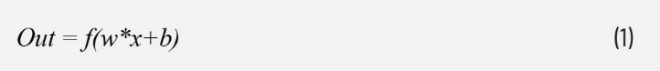
Where Out is the output, f is the activation function, w is the weight, x is the input data, and b is the bias. Data can be presented as a single scalar, vector, or matrix. Figure 1 shows a neuron with three inputs and a ReLU activation function. Neurons in the network are always arranged in layers.
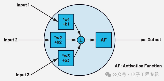
Figure 1: The structure of a neuron with three inputs and one output. (Data source: ADI)
As mentioned earlier, cellular neural networks are used for recognizing and classifying patterns in the input data. Cellular neural networks are divided into different parts: an input layer, several hidden layers, and an output layer. In Figure 2, a small network with three inputs, a hidden layer with five neurons, and an output layer with four outputs can be seen. All neuron outputs are connected to all inputs in the next layer. The network shown in Figure 2 is for demonstration purposes only and cannot handle any meaningful tasks. However, even for such a small demonstration network, the equations used to describe the network can have as many as 32 biases and 32 weights.
The CIFAR neural network is a CNN widely used for image recognition tasks. It consists of two main types of layers: convolutional layers and pooling layers. Both types of layers play a significant role in the training of neural networks. The convolutional layers use a mathematical operation called convolution to identify patterns in an array of pixel values. Convolution is implemented in the hidden layers, as shown in Figure 3. This process is repeated multiple times until the desired accuracy level is achieved. Note that if two input values to be compared (usually required for image processing and filtering) are similar, the output value of the convolution operation will always be particularly high. This is called a filter matrix, also known as a filter kernel or filter. The results are then passed to the pooling layer, which generates feature maps that characterize the data and can identify important features of the input data. This is also considered another filter matrix. In network operation, after training, these feature maps are compared with the input data. Since the feature maps contain object-specific type features, they will only trigger the output of the neurons when compared with the input images if the contents are similar. By combining these two methods, the CIFAR network can be used for high-precision recognition and classification of various objects in images.
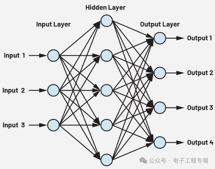
Figure 2: A small neural network.
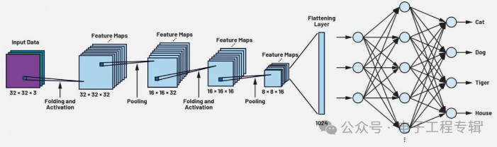
Figure 3: The CIFAR network model trained with the CIFAR-10 dataset.
CIFAR-10 is a specific dataset commonly used for training CIFAR neural networks. It consists of 60,000 32×32 color images. These images are divided into 10 major categories, collected from various sources such as web pages, newsgroups, and personal image collections. Each major category has 6,000 images, evenly divided into training, testing, and validation sets, making it an ideal set for testing new computer vision architectures and other machine learning models.
The main difference between CNNs and other types of networks lies in how they process data. By filtering, the properties of the input data are examined sequentially. As the number of concatenated convolutional layers increases, the level of detail recognition also increases. The process is: after the first convolution, it starts with the recognition of simple object attributes, such as edges or points; after the second convolution, it continues to more detailed structures, such as angles, circles, rectangles, etc.; and after the third convolution, the feature representation resembles complex patterns of parts of objects in the image, which are usually unique to a given object class (for example, in the initial case, these features are the cat’s whiskers or ears). In Figure 4, it can be seen that for the application itself, the visualization of feature maps is unnecessary, but it helps in understanding convolutions.
Even small networks like CIFAR are composed of many layers concatenated together, with the number of neurons in each layer reaching hundreds. As the complexity and scale of the network increase, the number of required weights and biases will increase rapidly. In the CIFAR-10 example shown in Figure 3, during training, the number of parameters required to determine a set of values has reached as many as 200,000. The pooling layers can further process the feature maps, reducing the number of parameters required for training while still retaining important information.
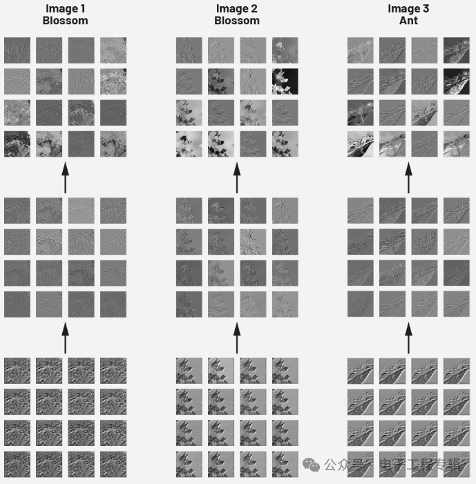
Figure 4: CNN Function Diagram.
As mentioned earlier, after each convolution in CNN, merging usually occurs, which is also called subsampling. This helps to reduce the dimensionality of the data. If we take a closer look at the feature map shown in Figure 4, we will notice that there is almost no meaningful information contained in larger areas. This is because the object does not constitute the entire image but occupies only a small part of it. This feature map does not take into account the rest of the image, hence it is irrelevant to classification recognition. In the pooling layer, the type of pooling (max or average) and the size of the window matrix are specified. During pooling, the window matrix moves over the input data in a stepwise manner. For example, in max pooling, the maximum data value in the window is taken, and all other values are discarded. In this way, the amount of data is continuously reduced, and eventually, it forms the unique attributes of the corresponding object class along with the convolution.
However, the results of these groups of convolutions and poolings are large two-dimensional matrices. To achieve classification recognition of practical goals, the two-dimensional data is converted into a longer one-dimensional vector. The conversion is done in a so-called flattening layer, followed by one or two fully connected layers. The neurons in the last two types of layers are similar to the structure shown in Figure 2. The output number of the last layer of this neural network corresponds exactly to the number of categories to be distinguished. Additionally, in the last layer, to adopt a probability distribution (97.5% cat, 2.1% leopard, 0.4% tiger, etc.), the data is also normalized.
At this point, the neural network modeling is complete. However, the weights of the kernel matrix and filter matrix, as well as their contents, remain unknown and must be determined through network training before the model can work. Utilizing the MAX78000AI microcontroller and a hardware-based CNN accelerator developed by ADI, a hardware solution for this neural network (for example, recognizing objects like cats) can be achieved.