Exploring Similarities Between Transformer, RNN, and SSM

Source: DeepHub IMBA

This article is approximately 4000 words long and is recommended to be read in 6 minutes.
This article will explore Transformer, RNN, and Mamba 2.

By exploring the potential connections between seemingly unrelated large language model (LLM) architectures, we may open new avenues for facilitating the exchange of ideas between different models and enhancing overall efficiency.Although linear recurrent neural networks (RNNs) and state space models (SSM) like Mamba have recently gained attention, the Transformer architecture remains a major pillar of LLMs. This pattern may soon change: hybrid architectures like Jamba, Samba, and Griffin show great potential. These models significantly outperform Transformers in terms of time and memory efficiency, while not showing a significant decline in capability compared to attention-based LLMs.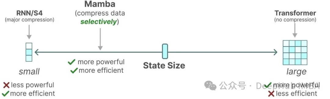Recent research has revealed deep connections between different architectural choices, including Transformers, RNNs, SSMs, and matrix mixers. This finding is significant as it opens possibilities for idea transfer between different architectures. This article will delve into Transformer, RNN, and Mamba 2, aiming to understand the following points through detailed algebraic analysis:

• Transformers can be viewed as RNNs in certain cases (Section 2)

• State space models may be hidden within the masks of self-attention mechanisms (Section 4)

• Mamba can be rewritten as masked self-attention under specific conditions (Section 5)

These connections are not only intriguing but may also have profound implications for future model design.

Masked Self-Attention Mechanism in LLMs

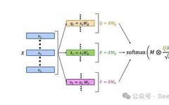
First, let’s review the structure of the classic LLM self-attention layer: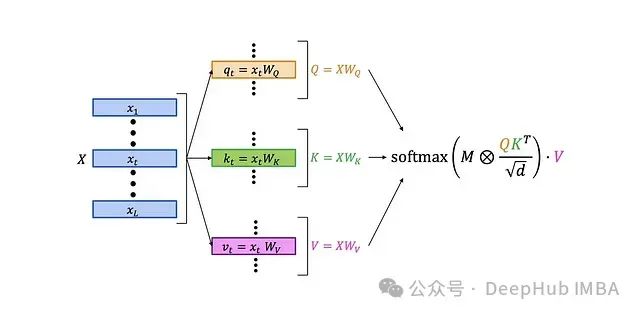The detailed structure is as follows: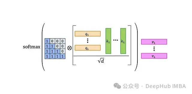The workflow of the self-attention layer is as follows:

• Multiply the query matrix Q by the key matrix K to obtain an L×L matrix containing the scalar products of queries and keys.

• Normalize the resulting matrix.

• Element-wise multiply the normalized matrix with an L×L attention mask. The diagram shows the default causal mask—the 0-1 matrix on the left. This step zeros out the products of earlier queries with later keys, preventing the attention mechanism from “seeing the future”.

• Apply the softmax function to the results.

• Finally, multiply the attention weight matrix A with the value matrix V. The output’s t-th row can be expressed as:

This means the i-th value is weighted by the “attention weight of the t-th query to the i-th key”.Many design choices in this architecture could be modified. Next, we will explore some possible variants.

Linearized Attention

The softmax function in the attention formula ensures that values are mixed with positive coefficients that sum to 1. This design preserves certain statistical properties but also brings limitations. For example, even if we want to utilize the associative law, such as (QK^T)V = Q(K^TV), we cannot break through the limitations of softmax.Why is the associative law so important? Because changing the order of multiplication can significantly affect computational complexity: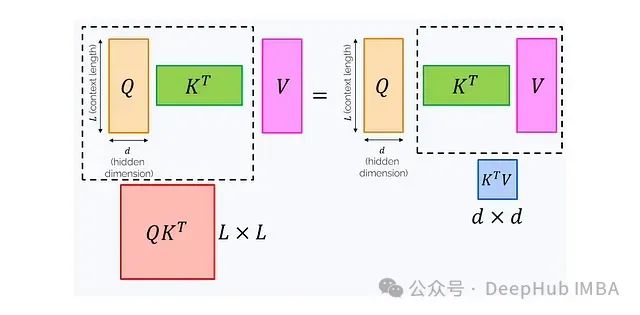The left-side formula requires calculating an L×L matrix, which has a complexity of O(L²d) and a memory consumption of O(L²) if this matrix is fully realized in memory. The right-side formula requires calculating a d×d matrix, with a complexity of O(Ld²) and a memory consumption of O(d²).As the context length L increases, the computational cost of the left-side formula rapidly becomes prohibitively high. To address this issue, we can consider removing softmax. Expanding the formula with softmax:Where:is the softmax function. The exponential function is the main obstacle that prevents us from extracting any terms from it. If we directly remove the exponential function:Then the normalization factorwill also disappear.This simplified formula has a problem: q_t^T k_s cannot guarantee to be positive, which may lead to values being mixed with coefficients of different signs, which is theoretically unreasonable. Worse, the denominator may be zero, leading to computational breakdown. To mitigate this issue, we can introduce a “good” element-wise function φ (called a kernel function):The original research suggests using φ(x) = 1 + elu(x) as the kernel function.This variant of the attention mechanism is called linearized attention. One important advantage is that it allows us to utilize the associative law:The relationship between M, K^T, and V in parentheses now becomes quite complex, no longer merely ordinary matrix multiplication and element-wise multiplication. We will discuss this computational unit in detail in the next section.If M is a causal mask, meaning that the diagonal and below are 1 and above the diagonal are 0:Then the computation can be further simplified:This can be computed through a simple recursive way: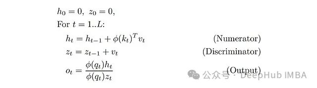This was first proposed in the 2020 ICML paper “Transformers are RNNs”. In this formula, we have two hidden states: vector z_t and matrix h_t (φ(k_t)^T v_t is a column vector multiplied by a row vector, resulting in a d×d matrix).Recent research often presents linearized attention in a more simplified form, removing the φ function and the denominator:Linearized attention has two main advantages:

• As a recursive mechanism, it has linear complexity relative to sequence length L during inference.

• As a Transformer model, it can be efficiently trained in parallel.

But you may ask: if linearized attention is so excellent, why hasn’t it been widely adopted in all LLMs? Are we discussing the issue of secondary complexity in attention? In fact, LLMs based on linearized attention have lower stability during training and slightly inferior capability compared to standard self-attention. This may be because the fixed d×d shape bottleneck conveys less information than the adjustable L×L shape bottleneck.

Further Exploration

The connection between RNNs and linearized attention has been rediscovered and explored in several recent studies. A common pattern is to use a matrix hidden state with the following update rule:Where k_t and v_t can be seen as some kind of “key” and “value”, the output form of the RNN layer is:This is essentially equivalent to linear attention. The following two papers provide some interesting examples:1. xLSTM (May 2024): This paper proposes improvements to the famous LSTM recurrent architecture. Its mLSTM block contains a matrix hidden state, with the update method as follows:The output is obtained by multiplying this state with a “query”. (Note: The linear algebra setup in this paper is opposite to ours, where queries, keys, and values are column vectors rather than row vectors, so the order of v_t k_t^T may look a bit strange.)2. Learning to (learn at test time) (July 2024): This is another RNN architecture with a matrix hidden state, where its hidden state W is a parameter of a function optimized through gradient descent during the iterations at t: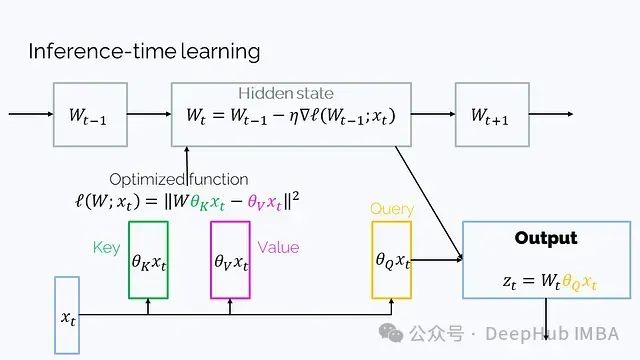The setup here is also transposed, so the order may look a bit different. Although the mathematical expression is more complex than W_t = W_{t-1} + v_t k_t^T, it can be simplified to this form.We have detailed both papers, and those interested can search for them independently.

Attention Masks

After simplifying the masked attention mechanism, we can begin to explore its potential development directions. An obvious research direction is to choose different lower triangular matrices (ensuring not to “see the future”) as the mask M, rather than simply using a 0-1 causal mask. Before embarking on this exploration, we need to address the efficiency issues it brings.In the previous section, we used a simple 0-1 causal mask M, which made recursive computation possible. But in general, this recursive trick is no longer applicable: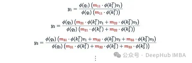The coefficient m_ts is no longer the same, and there is no simple recursive formula to relate y_3 to y_2. Therefore, for each t, we need to compute the total sum from scratch, which makes the computational complexity quadratic again rather than linear.The key to solving this problem is that we cannot use arbitrary masks M, but should choose special, “good” masks. We need those that can quickly multiply with other matrices (note that this is not element-wise multiplication). To understand how to benefit from this property, let’s analyze how to compute efficiently:First, clarify the meaning of this expression: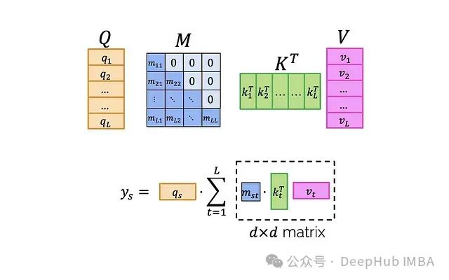If we delve into individual index levels:To facilitate subsequent discussions, we can mark the indices with different colors instead of blocks: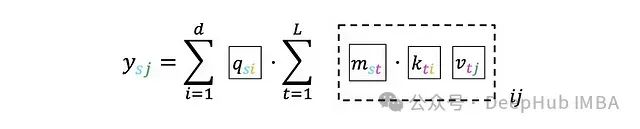Now we can propose a four-step algorithm:Step 1. Create a three-dimensional tensor Z using K and V, where: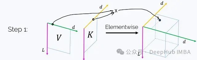(Each axis is labeled with its length.) This step requires O(Ld²) time and memory complexity. Notably, if we sum over the magenta axis t on this tensor, we will obtain the matrix product K^T V:Step 2. Multiply M by this tensor (note that this is not element-wise multiplication). M multiplies Z along each “column” of the magenta axis t.This yields:Let’s denote this result as H. Next, we just need to multiply everything by q, which will be done in the next two steps.Step 3a. Take Q and perform element-wise multiplication with each j = const layer of H:This will yield:This step requires O(Ld²) time and memory complexity.Step 3b. Sum the resulting tensor along the i-axis: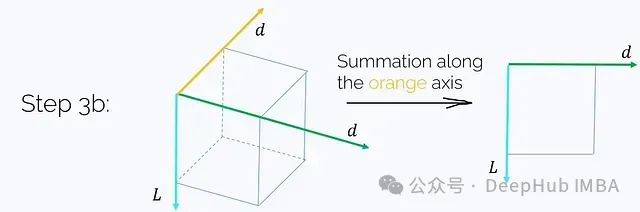This step also requires O(Ld²) time and memory complexity. Finally, we obtain the desired result:In this process, the most crucial part is the second step, where we intentionally omitted its complexity analysis. A simple estimate is:Each matrix multiplication requires O(L²) complexity, repeated d² timesThis would lead to a huge O(L²d²) complexity. However, our goal is to choose special M, so that multiplying M by a vector has a complexity of O(RL), where R is some not too large constant.For example, if M is a 0-1 causal matrix, then multiplying it actually corresponds to computing a cumulative sum, which can be done in O(L) time. But there are many other structured matrix options with rapid vector multiplication characteristics.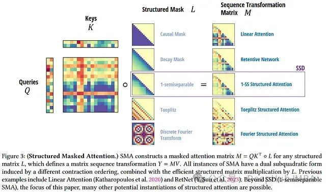In the next section, we will discuss an important example of this type of matrix—a semi-separable matrix, which has close ties to state space models.

Semi-Separable Matrices and State Space Models

Let’s review the definition of (discretized) state space models (SSM). SSM is a class of sequential models connecting 1D input x_t, r-dimensional hidden state h_t, and 1D output u_t, mathematically expressed as:In discrete form, SSM is essentially a complex linear RNN with skip connections. To simplify subsequent discussions, we can even ignore the skip connections by setting D_t = 0.Let’s represent SSM as a single matrix multiplication:WhereM is a lower triangular matrix, similar to the attention masks we discussed earlier.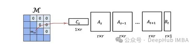This type of matrix has an important advantage:A lower triangular matrix of size L × L, if its elements can be represented in this way, can be stored using O(rL) memory and has a matrix-vector multiplication complexity of O(rL), rather than the default O(L²).This means that each state space model corresponds to a structured attention mask M, which can be used in an efficient Transformer model with linearized attention.Even without the surrounding query-key-value mechanism, the semi-separable matrix M itself is already quite complex and expressive. It itself may serve as a masked attention mechanism. We will explore this in detail in the next section.

State Space Duality

Here, we will introduce a core result from the Mamba 2 paper.Let’s consider again y = Mu, where u = u(x) is a function of the input, and M is a separable matrix. If we consider a very special case where each A_t is a scalar matrix: A_t = a_t I. In this case, the formula becomes particularly simple:Here,is just a scalar. We can also stack C_i and B_i into matrices B and C such that: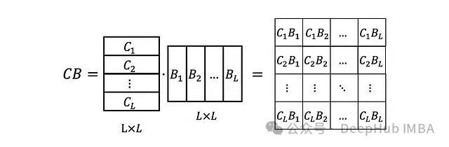Now we also need to define the matrix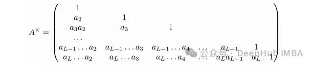Then it can be easily verified:Does this expression look familiar? This is actually a masked attention mechanism, where:

• G serves as the mask

• C serves as the query matrix Q

• B serves as the transposed key matrix K^T

• u serves as the value matrix V

In the classic SSM, B and C are constants. But in the Mamba model, they are designed to depend on the data, further reinforcing the correspondence with the attention mechanism. This specific correspondence between the state space model and masked attention is referred to as state space duality in the Mamba 2 paper.

Further Exploration

Using matrix mixers instead of more complex architectures is not a brand new idea. An early example is MLP-Mixer, which uses MLP instead of convolutions or attention for spatial mixing in computer vision tasks.Although current research primarily focuses on large language models (LLMs), some papers have proposed non-Transformer, matrix mixing architectures for encoder models. For example:

• FNet from Google Research, whose matrix mixer M is based on Fourier transforms.

• Hydra, which also proposes adaptive schemes for semi-separable matrices in non-causal (non-triangular) working modes, among other innovations.

Conclusion

This article delves into the potential connections between Transformers, recurrent neural networks (RNNs), and state space models (SSMs). The article first reviews the traditional masked self-attention mechanism, then introduces the concept of linearized attention, explaining its computational efficiency advantages. It then discusses the optimization of attention masks, introduces the concept of semi-separable matrices, and elaborates on their relationship with state space models. Finally, it introduces state space duality, revealing the correspondence between specific state space models and masked attention. Through these analyses, it shows that there are deep connections between seemingly different model architectures, providing new perspectives and possibilities for future model design and cross-architecture idea exchange.Author: Stanislav FedotovEditor: Huang Jiyan

About Us

Data Hub THU, as a public account for data science, backed by Tsinghua University’s Big Data Research Center, shares cutting-edge data science and big data technology innovation research dynamics, continuously disseminates data science knowledge, and strives to build a platform for data talent aggregation, creating the strongest group of big data in China.

Sina Weibo: @数据派THU

WeChat Video Account: 数据派THU

Today’s Headlines: 数据派THU